深度学习笔记(二)：简单神经网络，后向传播算法及实现

在之前的深度学习笔记(一):logistic分类中，已经描述了普通logistic回归以及如何将logistic回归用于多类分类。在这一节，我们再进一步，往其中加入隐藏层，构建出最简单的神经网络2.简单神经网络及后向传播算法2.1 大概描述和公式表达神经网络的大概结构如图所示，从左往右，分别是输入层，隐藏层，输出层，分别记为x\mathbf x,h\mathbf h, y\mathb

multiangle

17506人浏览 · 2016-09-16 22:31:45

multiangle · 2016-09-16 22:31:45 发布

深度学习笔记(一)：logistic分类
 深度学习笔记(二)：简单神经网络，后向传播算法及实现
 深度学习笔记(三)：激活函数和损失函数
 深度学习笔记：优化方法总结(BGD,SGD,Momentum,AdaGrad,RMSProp,Adam)
深度学习笔记(四)：循环神经网络的概念，结构和代码注释
 深度学习笔记(五)：LSTM
深度学习笔记(六)：Encoder-Decoder模型和Attention模型

在之前的深度学习笔记(一):logistic分类中，已经描述了普通logistic回归以及如何将logistic回归用于多类分类。在这一节，我们再进一步，往其中加入隐藏层，构建出最简单的神经网络

2.简单神经网络及后向传播算法

2.1 大概描述和公式表达

神经网络的大概结构如图所示，

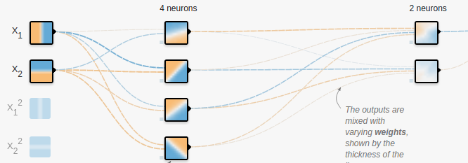
从左往右，分别是输入层，隐藏层，输出层，分别记为

x <script type="math/tex" id="MathJax-Element-22">\mathbf x</script>,

h <script type="math/tex" id="MathJax-Element-23">\mathbf h</script>,

y <script type="math/tex" id="MathJax-Element-24">\mathbf y</script>. 从输入层到隐藏层的矩阵记为

Whx <script type="math/tex" id="MathJax-Element-25">W_{hx}</script>, 偏置向量

bh <script type="math/tex" id="MathJax-Element-26">b_h</script>; 从隐藏层到输出层的矩阵记为

Wyh <script type="math/tex" id="MathJax-Element-27">W_{yh}</script>, 偏置向量为

by <script type="math/tex" id="MathJax-Element-28">b_y</script>. 那么根据之前logistic分类的公式稍作扩展，不难得到

h z = W h x x + b h h a = σ (h z) y z = W y h h a + b y y a = σ (y z)

ya <script type="math/tex" id="MathJax-Element-30"> \mathbf y_a</script> 以后的判断方法也比较类似，哪项最高就判定属于哪一类。真正值得写一下的是神经网络中的后向算法。按照传统的logistic分类，只能做到根据误差来更新

Wyh <script type="math/tex" id="MathJax-Element-31">W_{yh}</script> 和

by <script type="math/tex" id="MathJax-Element-32">\mathbf b_y</script> 那么如何来更新从输入层到隐藏层的参数

Whx <script type="math/tex" id="MathJax-Element-33">W_{hx}</script>和

bh <script type="math/tex" id="MathJax-Element-34">\mathbf b_h</script>呢？这就要用到后向算法了。所谓后向算法，就是指误差由输出层逐层往前传递，进而逐层更新参数矩阵和偏执向量。后向算法的核心其实就4个字：链式法则。首先来看

Wyh <script type="math/tex" id="MathJax-Element-35">W_{yh}</script> 和

by <script type="math/tex" id="MathJax-Element-36">\mathbf b_y</script>的更新

C = 1 2 (y a - y) 2 \partial C \partial y z = C' σ' (y z) = (y a - y) . \times a . \times (1 - a) \partial C \partial W y h = \partial C \partial y z \partial y z \partial W y h = C' σ' (y z) h T a \partial C \partial b y = \partial C \partial y z \partial y z \partial b y = C' σ' (y z)

\partial C \partial h a = \partial C \partial y z \partial y z \partial h a = W T y h [C' σ' (y z)] \partial C \partial W h x = \partial C \partial h a \partial h a \partial W = [\partial C \partial h a σ' (h z)] x T \partial C \partial b h = \partial C \partial h a \partial h a \partial b h = [\partial C \partial h a σ' (h z)]

Whx <script type="math/tex" id="MathJax-Element-39">W_{hx}</script>和

bh <script type="math/tex" id="MathJax-Element-40">\mathbf b_h</script>的计算中都用到了

∂C∂ha <script type="math/tex" id="MathJax-Element-41"> \frac{\partial C}{\partial \mathbf h_a}</script> 这可以看成由输出层传递到中间层的误差。那么在获得了各参数的偏导数以后，就可以对参数进行修正了

W y h : = W y h - η \partial C \partial W y h b y : = b y - η \partial C \partial b y W h x : = W h x - η \partial C \partial W h x b h : = b h - η \partial C \partial b h

2.2 神经网络的简单实现

为了加深印象，我自己实现了一个神经网络分类器，分类效果如下图所示

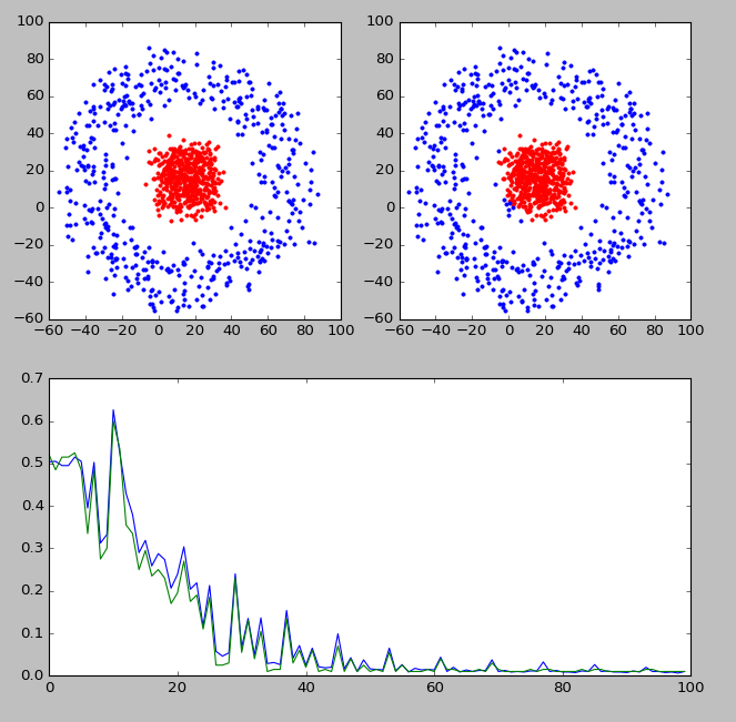
上图中，左上角显示的是实际的分类，右上角显示的是分类器判断出的各点分类。靠下的图显示的是分类器的判断准确率随迭代次数的变化情况。可以看到，经过训练以后，分类器的判断准确率还是可以的。

下面是代码部分

import numpy as np
import matplotlib.pyplot as plt
import random
import math


# 构造各个分类
def gen_sample():
    data = []
    radius = [0,50]
    for i in range(1000):  # 生成10k个点
        catg = random.randint(0,1)  # 决定分类
        r = random.random()*10
        arg = random.random()*360
        len = r + radius[catg]
        x_c = math.cos(math.radians(arg))*len
        y_c = math.sin(math.radians(arg))*len
        x = random.random()*30 + x_c
        y = random.random()*30 + y_c
        data.append((x,y,catg))
    return data

def plot_dots(data):
    data_asclass = [[] for i in range(2)]
    for d in data:
        data_asclass[int(d[2])].append((d[0],d[1]))
    colors = ['r.','b.','r.','b.']
    for i,d in enumerate(data_asclass):
        # print(d)
        nd = np.array(d)
        plt.plot(nd[:,0],nd[:,1],colors[i])
    plt.draw()

def train(input, output, Whx, Wyh, bh, by):
    """
    完成神经网络的训练过程
    :param input:   输入列向量， 例如 [x,y].T
    :param output:  输出列向量, 例如[0,1,0,0].T
    :param Whx:     x->h 的参数矩阵
    :param Wyh:     h->y 的参数矩阵
    :param bh:      x->h 的偏置向量
    :param by:      h->y 的偏置向量
    :return:
    """
    h_z = np.dot(Whx, input) + bh   # 线性求和
    h_a = 1/(1+np.exp(-1*h_z))      # 经过sigmoid激活函数
    y_z = np.dot(Wyh, h_a) + by
    y_a = 1/(1+np.exp(-1*y_z))
    c_y = (y_a-output)*y_a*(1-y_a)
    dWyh = np.dot(c_y, h_a.T)
    dby = c_y
    c_h = np.dot(Wyh.T, c_y)*h_a*(1-h_a)
    dWhx = np.dot(c_h,input.T)
    dbh = c_h
    return dWhx,dWyh,dbh,dby,c_y

def test(train_set, test_set, Whx, Wyh, bh, by):
    train_tag = [int(x) for x in train_set[:,2]]
    test_tag = [int(x) for x in test_set[:,2]]
    train_pred = []
    test_pred = []

    for i,d in enumerate(train_set):
        input = train_set[i:i+1,0:2].T
        tag = predict(input,Whx,Wyh,bh,by)
        train_pred.append(tag)
    for i,d in enumerate(test_set):
        input = test_set[i:i+1,0:2].T
        tag = predict(input,Whx,Wyh,bh,by)
        test_pred.append(tag)
    # print(train_tag)
    # print(train_pred)
    train_err = 0
    test_err = 0
    for i in range(train_pred.__len__()):
        if train_pred[i]!=int(train_tag[i]):
            train_err += 1
    for i in range(test_pred.__len__()):
        if test_pred[i]!=int(test_tag[i]):
            test_err += 1
    # print(test_tag)
    # print(test_pred)
    train_ratio = train_err / train_pred.__len__()
    test_ratio = test_err / test_pred.__len__()
    return train_err,train_ratio,test_err,test_ratio

def predict(input,Whx,Wyh,bh,by):
    # print('-----------------')
    # print(input)
    h_z = np.dot(Whx, input) + bh   # 线性求和
    h_a = 1/(1+np.exp(-1*h_z))      # 经过sigmoid激活函数
    y_z = np.dot(Wyh, h_a) + by
    y_a = 1/(1+np.exp(-1*y_z))
    # print(y_a)
    tag = np.argmax(y_a)
    return tag



if __name__=='__main__':
    input_dim   = 2
    output_dim  = 2
    hidden_size = 200
    Whx = np.random.randn(hidden_size, input_dim)*0.01
    Wyh = np.random.randn(output_dim, hidden_size)*0.01
    bh  = np.zeros((hidden_size, 1))
    by  = np.zeros((output_dim, 1))
    data = gen_sample()
    plt.subplot(221)
    plot_dots(data)
    ndata = np.array(data)
    train_set = ndata[0:800,:]
    test_set = ndata[800:1000,:]
    train_ratio_list = []
    test_ratio_list = []
    for times in range(10000):
        i = times%train_set.__len__()
        input = train_set[i:i+1,0:2].T
        tag = int(train_set[i,2])
        output = np.zeros((2,1))
        output[tag,0] = 1
        dWhx,dWyh,dbh,dby,c_y = train(input,output,Whx,Wyh,bh,by)
        if times%100==0:
            train_err,train_ratio,test_err,test_ratio = test(train_set,test_set,Whx,Wyh,bh,by)
            print('times:{t}\t train ratio:{tar}\t test ratio: {ter}'.format(tar=train_ratio,ter=test_ratio,t=times))
            train_ratio_list.append(train_ratio)
            test_ratio_list.append(test_ratio)

        for param, dparam in zip([Whx, Wyh, bh, by],
                                 [dWhx,dWyh,dbh,dby]):
            param -= 0.01*dparam
    for i,d in enumerate(ndata):
        input = ndata[i:i+1,0:2].T
        tag = predict(input,Whx,Wyh,bh,by)
        ndata[i,2] = tag
    plt.subplot(222)
    plot_dots(ndata)
    # plt.figure()
    plt.subplot(212)
    plt.plot(train_ratio_list)
    plt.plot(test_ratio_list)
    plt.show()