7.2 GaussianMixture实战
·
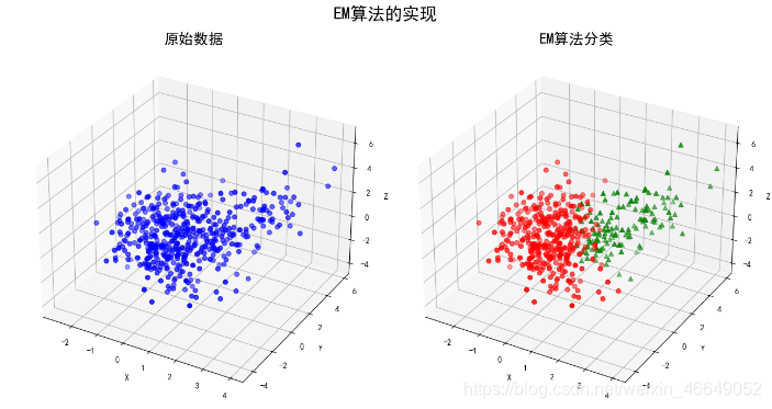
1.多维GMM聚类
#!usr/bin/env python
# -*- coding:utf-8 -*-
"""
@author: admin
@file: EM.py
@time: 2021/02/03
@desc:
"""

import numpy as np
from scipy.stats import multivariate_normal
from sklearn.mixture import GaussianMixture
import matplotlib as mpl
import matplotlib.pyplot as plt
from sklearn.metrics.pairwise import pairwise_distances_argmin


mpl.rcParams['font.sans-serif'] = [u'SimHei']
mpl.rcParams['axes.unicode_minus'] = False


if __name__ == '__main__':
    style = 'myself'

    np.random.seed(0)
    mu1_fact = (0, 0, 0)
    # np.diag((1, 2, 3))生成对角线数组,除对角线外,其余位置为0
    cov1_fact = np.diag((1, 2, 3))
    # 生成一个多元正态分布矩阵
    data1 = np.random.multivariate_normal(mu1_fact, cov1_fact, 400) # (400,3)
    mu2_fact = (2, 2, 1)
    cov2_fact = np.array(((1, 1, 3), (1, 2, 1), (0, 0, 1)))
    data2 = np.random.multivariate_normal(mu2_fact, cov2_fact, 100,check_valid='ignore') # (100,3)
    data = np.vstack((data1, data2))
    y = np.array([True] * 400 + [False] * 100)

    if style == 'sklearn':
        # n_components表示混合高斯模型的个数
        # covariance_type描述协方差的类型;默认‘full’ ,完全协方差矩阵
        # tol:EM迭代停止阈值,默认为1e-3.
        # max_iter:最大迭代次数,默认100
        gm = GaussianMixture(n_components=2, covariance_type='full', tol=1e-6, max_iter=1000)
        gm.fit(data)
        print('类别概率:\t', gm.weights_[0])
        print('均值:\n', gm.means_, '\n')
        print('方差:\n', gm.covariances_, '\n')
        mu1, mu2 = gm.means_
        sigma1, sigma2 = gm.covariances_
    else:
        num_iter = 100
        n, d = data.shape
        # 随机指定
        # mu1 = np.random.standard_normal(d)
        # print mu1
        # mu2 = np.random.standard_normal(d)
        # print mu2
        mu1 = data.min(axis=0)
        mu2 = data.max(axis=0)
        sigma1 = np.identity(d)
        sigma2 = np.identity(d)
        pi = 0.5
        # EM
        for i in range(num_iter):
            # E Step
            norm1 = multivariate_normal(mu1, sigma1)
            norm2 = multivariate_normal(mu2, sigma2)
            tau1 = pi * norm1.pdf(data)
            tau2 = (1 - pi) * norm2.pdf(data)
            gamma = tau1 / (tau1 + tau2)

            # M Step
            mu1 = np.dot(gamma, data) / np.sum(gamma)
            mu2 = np.dot((1 - gamma), data) / np.sum((1 - gamma))
            sigma1 = np.dot(gamma * (data - mu1).T, data - mu1) / np.sum(gamma)
            sigma2 = np.dot((1 - gamma) * (data - mu2).T, data - mu2) / np.sum(1 - gamma)
            pi = np.sum(gamma) / n
            print(i, ":\t", mu1, mu2)
        print('类别概率:\t', pi)
        print('均值:\t', mu1, mu2)
        print('方差:\n', sigma1, '\n\n', sigma2, '\n')

    # 预测分类
    norm1 = multivariate_normal(mu1, sigma1)
    norm2 = multivariate_normal(mu2, sigma2)
    tau1 = norm1.pdf(data)
    tau2 = norm2.pdf(data)


    fig = plt.figure(figsize=(13, 7), facecolor='w')
    ax = fig.add_subplot(121, projection='3d')
    ax.scatter(data[:, 0], data[:, 1], data[:, 2], c='b', s=30, marker='o', depthshade=True)
    ax.set_xlabel('X')
    ax.set_ylabel('Y')
    ax.set_zlabel('Z')
    ax.set_title(u'原始数据', fontsize=18)
    ax = fig.add_subplot(122, projection='3d')
    order = pairwise_distances_argmin([mu1_fact, mu2_fact], [mu1, mu2], metric='euclidean')
    print(order)
    if order[0] == 0:
        c1 = tau1 > tau2
    else:
        c1 = tau1 < tau2
    c2 = ~c1
    acc = np.mean(y == c1)
    print(u'准确率:%.2f%%' % (100*acc))
    ax.scatter(data[c1, 0], data[c1, 1], data[c1, 2], c='r', s=30, marker='o', depthshade=True)
    ax.scatter(data[c2, 0], data[c2, 1], data[c2, 2], c='g', s=30, marker='^', depthshade=True)
    ax.set_xlabel('X')
    ax.set_ylabel('Y')
    ax.set_zlabel('Z')
    ax.set_title(u'EM算法分类', fontsize=18)
    plt.suptitle(u'EM算法的实现', fontsize=21)
    plt.subplots_adjust(top=0.90)
    plt.tight_layout()
    plt.show()
# !/usr/bin/python
# -*- coding:utf-8 -*-

import numpy as np
from sklearn.mixture import GaussianMixture
from sklearn.model_selection import train_test_split
import matplotlib as mpl
import matplotlib.colors
import matplotlib.pyplot as plt

mpl.rcParams['font.sans-serif'] = [u'SimHei']
mpl.rcParams['axes.unicode_minus'] = False


# from matplotlib.font_manager import FontProperties
# font_set = FontProperties(fname=r"c:\windows\fonts\simsun.ttc", size=15)
# fontproperties=font_set


def expand(a, b):
    d = (b - a) * 0.05
    return a - d, b + d


if __name__ == '__main__':
    data = np.loadtxt('HeightWeight.csv', dtype=np.float, delimiter=',', skiprows=1)
    print(data.shape)
    y, x = np.split(data, [1, ], axis=1)
    x, x_test, y, y_test = train_test_split(x, y, train_size=0.6, random_state=0)
    gmm = GaussianMixture(n_components=2, covariance_type='full', random_state=0)
    gmm.fit(x)
    print('均值 = \n', gmm.means_)
    print('方差 = \n', gmm.covariances_)
    y_hat = gmm.predict(x)
    y_test_hat = gmm.predict(x_test)

    x_min = np.min(x, axis=0)
    x_max = np.max(x, axis=0)
    # 确保类1的身高高于类2
    change = (gmm.means_[0][0] > gmm.means_[1][0])
    if change:
        z = y_hat == 0
        y_hat[z] = 1
        y_hat[~z] = 0
        z = y_test_hat == 0
        y_test_hat[z] = 1
        y_test_hat[~z] = 0
    acc = np.mean(y_hat.ravel() == y.ravel())
    acc_test = np.mean(y_test_hat.ravel() == y_test.ravel())
    acc_str = u'训练集准确率:%.2f%%' % (acc * 100)
    acc_test_str = u'测试集准确率:%.2f%%' % (acc_test * 100)
    print(acc_str)
    print(acc_test_str)

    cm_light = mpl.colors.ListedColormap(['#FF8080', '#77E0A0'])
    cm_dark = mpl.colors.ListedColormap(['r', 'g'])
    # 画决策边界图
    x1_min, x1_max = x[:, 0].min(), x[:, 0].max()
    x2_min, x2_max = x[:, 1].min(), x[:, 1].max()
    x1_min, x1_max = expand(x1_min, x1_max)
    x2_min, x2_max = expand(x2_min, x2_max)
    x1, x2 = np.mgrid[x1_min:x1_max:500j, x2_min:x2_max:500j]
    grid_test = np.stack((x1.flat, x2.flat), axis=1)
    grid_hat = gmm.predict(grid_test)
    grid_hat = grid_hat.reshape(x1.shape)
    if change:
        z = grid_hat == 0
        grid_hat[z] = 1
        grid_hat[~z] = 0
    plt.figure(figsize=(9, 7), facecolor='w')
    plt.pcolormesh(x1, x2, grid_hat, cmap=cm_light, shading='auto')
    plt.scatter(x[:, 0], x[:, 1], s=50, c=y, marker='o', cmap=cm_dark, edgecolors='k')
    plt.scatter(x_test[:, 0], x_test[:, 1], s=60, c=y_test, marker='^', cmap=cm_dark, edgecolors='k')

    # 概率
    p = gmm.predict_proba(grid_test)
    print(p)
    p = p[:, 0].reshape(x1.shape)
    CS = plt.contour(x1, x2, p, levels=(0.1, 0.5, 0.8), colors=list('rgb'), linewidths=2)
    plt.clabel(CS, fontsize=15, fmt='%.1f', inline=True)
    ax1_min, ax1_max, ax2_min, ax2_max = plt.axis()
    xx = 0.9 * ax1_min + 0.1 * ax1_max
    yy = 0.1 * ax2_min + 0.9 * ax2_max
    plt.text(xx, yy, acc_str, fontsize=18)
    yy = 0.15 * ax2_min + 0.85 * ax2_max
    plt.text(xx, yy, acc_test_str, fontsize=18)
    plt.xlim((x1_min, x1_max))
    plt.ylim((x2_min, x2_max))
    plt.xlabel(u'身高(cm)', fontsize='large')
    plt.ylabel(u'体重(kg)', fontsize='large')
    plt.title(u'EM算法估算GMM的参数', fontsize=20)
    plt.grid()
    plt.show()

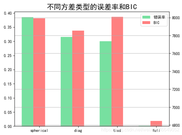
2.GMM调参
# !/usr/bin/python
# -*- coding:utf-8 -*-
import numpy as np
from sklearn.mixture import GaussianMixture
import matplotlib as mpl
import matplotlib.colors
import matplotlib.pyplot as plt
mpl.rcParams['font.sans-serif'] = [u'SimHei']
mpl.rcParams['axes.unicode_minus'] = False
def expand(a, b, rate=0.05):
d = (b - a) * rate
return a-d, b+d
def accuracy_rate(y1, y2):
acc = np.mean(y1 == y2)
return acc if acc > 0.5 else 1-acc
if __name__ == '__main__':
np.random.seed(0)
cov1 = np.diag((1, 2))
print(cov1)
N1 = 500
N2 = 300
N = N1 + N2
x1 = np.random.multivariate_normal(mean=(1, 2), cov=cov1, size=N1)
m = np.array(((1, 1), (1, 3)))
x1 = x1.dot(m)
x2 = np.random.multivariate_normal(mean=(-1, 10), cov=cov1, size=N2)
x = np.vstack((x1, x2))
y = np.array([0]*N1 + [1]*N2)
types = ('spherical', 'diag', 'tied', 'full')
err = np.empty(len(types))
bic = np.empty(len(types))
for i, type in enumerate(types):
gmm = GaussianMixture(n_components=2, covariance_type=type, random_state=0)
gmm.fit(x)
err[i] = 1 - accuracy_rate(gmm.predict(x), y)
bic[i] = gmm.bic(x)
print('错误率:', err.ravel())
print('BIC:', bic.ravel())
xpos = np.arange(4)
plt.figure(facecolor='w')
ax = plt.axes()
b1 = ax.bar(xpos-0.3, err, width=0.3, color='#77E0A0')
b2 = ax.twinx().bar(xpos, bic, width=0.3, color='#FF8080')
# print(b1[0])
plt.grid(True)
bic_min, bic_max = expand(bic.min(), bic.max())
plt.ylim((bic_min, bic_max))
plt.xticks(xpos, types)
plt.legend([b1[0], b2[0]], (u'错误率', u'BIC'))
plt.title(u'不同方差类型的误差率和BIC', fontsize=18)
plt.show()
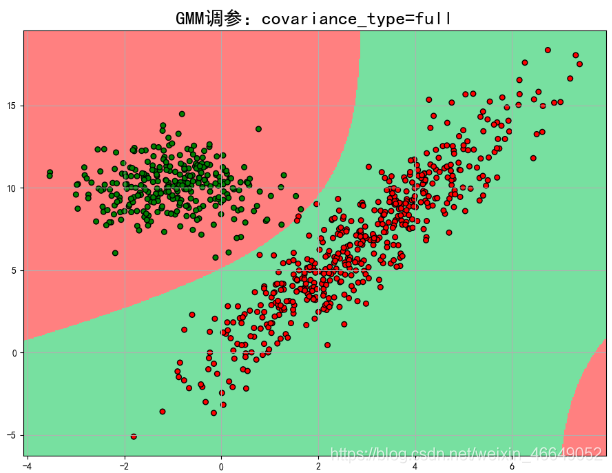
optimal = bic.argmin()
# print(optimal)
gmm = GaussianMixture(n_components=2, covariance_type=types[optimal], random_state=0)
gmm.fit(x)
print('均值 = \n', gmm.means_)
print('方差 = \n', gmm.covariances_)
y_hat = gmm.predict(x)
cm_light = mpl.colors.ListedColormap(['#FF8080', '#77E0A0'])
cm_dark = mpl.colors.ListedColormap(['r', 'g'])
x1_min, x1_max = x[:, 0].min(), x[:, 0].max()
x2_min, x2_max = x[:, 1].min(), x[:, 1].max()
x1_min, x1_max = expand(x1_min, x1_max)
x2_min, x2_max = expand(x2_min, x2_max)
x1, x2 = np.mgrid[x1_min:x1_max:500j, x2_min:x2_max:500j]
grid_test = np.stack((x1.flat, x2.flat), axis=1)
grid_hat = gmm.predict(grid_test)
grid_hat = grid_hat.reshape(x1.shape)
if gmm.means_[0][0] > gmm.means_[1][0]:
z = grid_hat == 0
grid_hat[z] = 1
grid_hat[~z] = 0
plt.figure(figsize=(9, 7), facecolor='w')
plt.pcolormesh(x1, x2, grid_hat, cmap=cm_light,shading='auto')
plt.scatter(x[:, 0], x[:, 1], s=30, c=y, marker='o', cmap=cm_dark, edgecolors='k')
ax1_min, ax1_max, ax2_min, ax2_max = plt.axis()
plt.xlim((x1_min, x1_max))
plt.ylim((x2_min, x2_max))
plt.title(u'GMM调参:covariance_type=%s' % types[optimal], fontsize=20)
plt.grid()
plt.show()
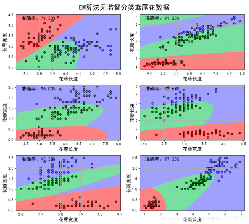
3. 鸢尾花数据集
import numpy as np
import pandas as pd
from sklearn.mixture import GaussianMixture
import matplotlib as mpl
import matplotlib.colors
import matplotlib.pyplot as plt
from sklearn.metrics.pairwise import pairwise_distances_argmin

mpl.rcParams['font.sans-serif'] = [u'SimHei']
mpl.rcParams['axes.unicode_minus'] = False

iris_feature = u'花萼长度', u'花萼宽度', u'花瓣长度', u'花瓣宽度'


def expand(a, b, rate=0.05):
    d = (b - a) * rate
    return a-d, b+d


if __name__ == '__main__':
    path = 'iris.data'
    data = pd.read_csv(path, header=None)
    x_prime, y = data[np.arange(4)], data[4]
    y = pd.Categorical(y).codes

    n_components = 3
    feature_pairs = [[0, 1], [0, 2], [0, 3], [1, 2], [1, 3], [2, 3]]
    plt.figure(figsize=(10, 9), facecolor='#FFFFFF')
    for k, pair in enumerate(feature_pairs):
        x = x_prime[pair]
        m = np.array([np.mean(x[y == i], axis=0) for i in range(3)])  # 均值的实际值
        print('实际均值 = \n', m)

        gmm = GaussianMixture(n_components=n_components, covariance_type='full', random_state=0)
        gmm.fit(x)
        print('预测均值 = \n', gmm.means_)
        print('预测方差 = \n', gmm.covariances_)
        y_hat = gmm.predict(x)
        order = pairwise_distances_argmin(m, gmm.means_, axis=1, metric='euclidean')
        # 实际对应标签
        print('顺序:\t', order)

        n_sample = y.size
        n_types = 3
        change = np.empty((n_types, n_sample), dtype=np.bool)
        # 交换顺序
        for i in range(n_types):
            change[i] = y_hat == order[i]
        for i in range(n_types):
            y_hat[change[i]] = i

        acc = u'准确率:%.2f%%' % (100*np.mean(y_hat == y))
        print(acc)

		# 画决策边界图
        cm_light = mpl.colors.ListedColormap(['#FF8080', '#77E0A0', '#A0A0FF'])
        cm_dark = mpl.colors.ListedColormap(['r', 'g', '#6060FF'])
        x1_min, x2_min = x.min()
        x1_max, x2_max = x.max()
        x1_min, x1_max = expand(x1_min, x1_max)
        x2_min, x2_max = expand(x2_min, x2_max)
        x1, x2 = np.mgrid[x1_min:x1_max:500j, x2_min:x2_max:500j]
        grid_test = np.stack((x1.flat, x2.flat), axis=1)
        grid_hat = gmm.predict(grid_test)

        change = np.empty((n_types, grid_hat.size), dtype=np.bool)
        for i in range(n_types):
            change[i] = grid_hat == order[i]
        for i in range(n_types):
            grid_hat[change[i]] = i

        grid_hat = grid_hat.reshape(x1.shape)
        plt.subplot(3, 2, k+1)
        plt.pcolormesh(x1, x2, grid_hat, cmap=cm_light)
        plt.scatter(x[pair[0]], x[pair[1]], s=30, c=y, marker='o', cmap=cm_dark, edgecolors='k')
        xx = 0.95 * x1_min + 0.05 * x1_max
        yy = 0.1 * x2_min + 0.9 * x2_max
        plt.text(xx, yy, acc, fontsize=14)
        plt.xlim((x1_min, x1_max))
        plt.ylim((x2_min, x2_max))
        plt.xlabel(iris_feature[pair[0]], fontsize=14)
        plt.ylabel(iris_feature[pair[1]], fontsize=14)
        plt.grid()
    plt.tight_layout(2)
    plt.suptitle(u'EM算法无监督分类鸢尾花数据', fontsize=20)
    plt.subplots_adjust(top=0.92)
    plt.show()
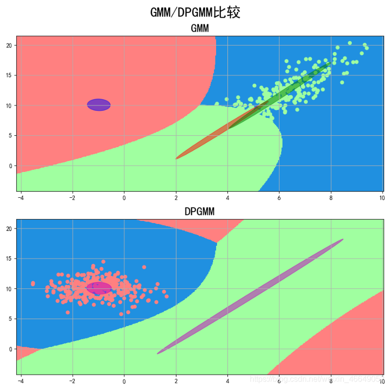
4.GMM与DPGMM比较
import numpy as np
from sklearn.mixture import GaussianMixture, BayesianGaussianMixture
import scipy as sp
import matplotlib as mpl
import matplotlib.colors
import matplotlib.pyplot as plt
from matplotlib.patches import Ellipse


def expand(a, b, rate=0.05):
    d = (b - a) * rate
    return a-d, b+d


matplotlib.rcParams['font.sans-serif'] = [u'SimHei']
matplotlib.rcParams['axes.unicode_minus'] = False


if __name__ == '__main__':
    np.random.seed(0)
    cov1 = np.diag((1, 2))
    N1 = 500
    N2 = 300
    N = N1 + N2
    x1 = np.random.multivariate_normal(mean=(3, 2), cov=cov1, size=N1)
    m = np.array(((1, 1), (1, 3)))
    # 点乘
    x1 = x1.dot(m)
    x2 = np.random.multivariate_normal(mean=(-1, 10), cov=cov1, size=N2)
    x = np.vstack((x1, x2))
    y = np.array([0]*N1 + [1]*N2)
    n_components = 3

    # 绘制决策边界图
    colors = '#A0FFA0', '#2090E0', '#FF8080'
    cm = mpl.colors.ListedColormap(colors)
    x1_min, x1_max = x[:, 0].min(), x[:, 0].max()
    x2_min, x2_max = x[:, 1].min(), x[:, 1].max()
    x1_min, x1_max = expand(x1_min, x1_max)
    x2_min, x2_max = expand(x2_min, x2_max)
    x1, x2 = np.mgrid[x1_min:x1_max:500j, x2_min:x2_max:500j]
    grid_test = np.stack((x1.flat, x2.flat), axis=1)

    plt.figure(figsize=(9, 9), facecolor='w')
    plt.suptitle(u'GMM/DPGMM比较', fontsize=23)

    ax = plt.subplot(211)
    gmm = GaussianMixture(n_components=n_components, covariance_type='full', random_state=0)
    gmm.fit(x)
    centers = gmm.means_
    covs = gmm.covariances_
    print('GMM均值 = \n', centers)
    print('GMM方差 = \n', covs)
    y_hat = gmm.predict(x)

    grid_hat = gmm.predict(grid_test)
    grid_hat = grid_hat.reshape(x1.shape)
    plt.pcolormesh(x1, x2, grid_hat, cmap=cm)
    plt.scatter(x[:, 0], x[:, 1], s=30, c=y, cmap=cm, marker='o')

    clrs = list('rgbmy')
    for i, (center, cov) in enumerate(zip(centers, covs)):
        value, vector = sp.linalg.eigh(cov)
        width, height = value[0], value[1]
        v = vector[0] / sp.linalg.norm(vector[0])
        angle = 180* np.arctan(v[1] / v[0]) / np.pi
        e = Ellipse(xy=center, width=width, height=height,
                    angle=angle, color=clrs[i], alpha=0.5, clip_box = ax.bbox)
        ax.add_artist(e)

    ax1_min, ax1_max, ax2_min, ax2_max = plt.axis()
    plt.xlim((x1_min, x1_max))
    plt.ylim((x2_min, x2_max))
    plt.title(u'GMM', fontsize=20)
    plt.grid(True)

    # DPGMM
    dpgmm = BayesianGaussianMixture(n_components=n_components, covariance_type='full', max_iter=1000, n_init=5,
                                    weight_concentration_prior_type='dirichlet_process', weight_concentration_prior=0.1)
    dpgmm.fit(x)
    centers = dpgmm.means_
    covs = dpgmm.covariances_
    print('DPGMM均值 = \n', centers)
    print('DPGMM方差 = \n', covs)
    y_hat = dpgmm.predict(x)
    print(y_hat)

    ax = plt.subplot(212)
    grid_hat = dpgmm.predict(grid_test)
    grid_hat = grid_hat.reshape(x1.shape)
    plt.pcolormesh(x1, x2, grid_hat, cmap=cm)
    plt.scatter(x[:, 0], x[:, 1], s=30, c=y, cmap=cm, marker='o')

    for i, cc in enumerate(zip(centers, covs)):
        if i not in y_hat:
            continue
        center, cov = cc
        value, vector = sp.linalg.eigh(cov)
        width, height = value[0], value[1]
        v = vector[0] / sp.linalg.norm(vector[0])
        angle = 180* np.arctan(v[1] / v[0]) / np.pi
        e = Ellipse(xy=center, width=width, height=height,
                    angle=angle, color='m', alpha=0.5, clip_box = ax.bbox)
        ax.add_artist(e)

    plt.xlim((x1_min, x1_max))
    plt.ylim((x2_min, x2_max))
    plt.title('DPGMM', fontsize=20)
    plt.grid(True)

    plt.tight_layout()
    plt.subplots_adjust(top=0.9)
    plt.show()
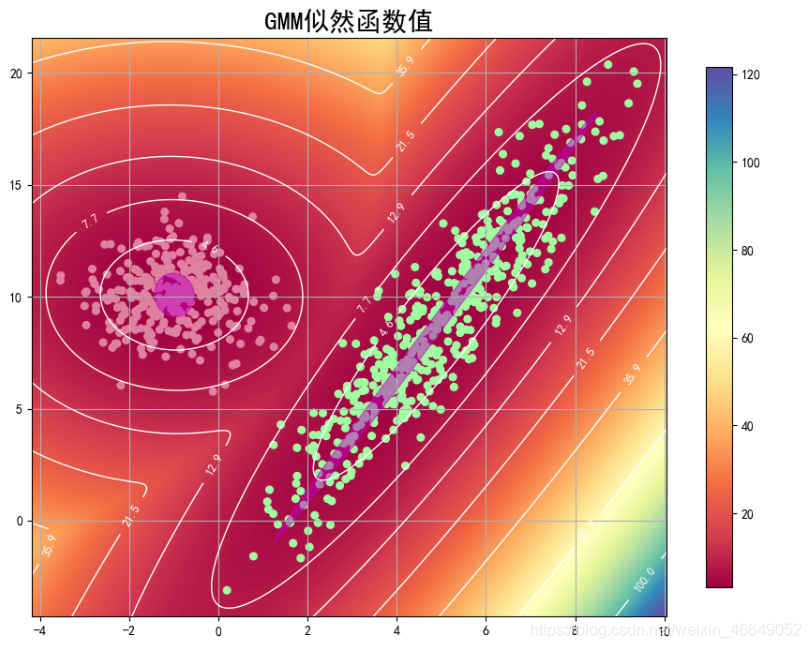
5. GMM似然函数值
import numpy as np
from sklearn.mixture import GaussianMixture
import scipy as sp
import matplotlib as mpl
import matplotlib.colors
import matplotlib.pyplot as plt
from matplotlib.patches import Ellipse
import warnings


def expand(a, b, rate=0.05):
    d = (b - a) * rate
    return a-d, b+d


if __name__ == '__main__':
    warnings.filterwarnings(action='ignore', category=RuntimeWarning)
    np.random.seed(0)
    cov1 = np.diag((1, 2))
    N1 = 500
    N2 = 300
    N = N1 + N2
    x1 = np.random.multivariate_normal(mean=(3, 2), cov=cov1, size=N1)
    m = np.array(((1, 1), (1, 3)))
    x1 = x1.dot(m)
    x2 = np.random.multivariate_normal(mean=(-1, 10), cov=cov1, size=N2)
    x = np.vstack((x1, x2))
    y = np.array([0]*N1 + [1]*N2)

    gmm = GaussianMixture(n_components=2, covariance_type='full', random_state=0)
    gmm.fit(x)
    centers = gmm.means_
    covs = gmm.covariances_
    print('GMM均值 = \n', centers)
    print('GMM方差 = \n', covs)
    y_hat = gmm.predict(x)

    colors = '#A0FFA0', '#E080A0',
    levels = 10
    cm = mpl.colors.ListedColormap(colors)
    x1_min, x1_max = x[:, 0].min(), x[:, 0].max()
    x2_min, x2_max = x[:, 1].min(), x[:, 1].max()
    x1_min, x1_max = expand(x1_min, x1_max)
    x2_min, x2_max = expand(x2_min, x2_max)
    x1, x2 = np.mgrid[x1_min:x1_max:500j, x2_min:x2_max:500j]
    grid_test = np.stack((x1.flat, x2.flat), axis=1)
    print(gmm.score_samples(grid_test))
    grid_hat = -gmm.score_samples(grid_test)
    grid_hat = grid_hat.reshape(x1.shape)
    plt.figure(figsize=(9, 7), facecolor='w')
    ax = plt.subplot(111)
    cmesh = plt.pcolormesh(x1, x2, grid_hat, cmap=plt.cm.Spectral)
    plt.colorbar(cmesh, shrink=0.9)
    CS = plt.contour(x1, x2, grid_hat, levels=np.logspace(0, 2, num=levels, base=10), colors='w', linewidths=1)
    plt.clabel(CS, fontsize=9, inline=True, fmt='%.1f')
    plt.scatter(x[:, 0], x[:, 1], s=30, c=y, cmap=cm, marker='o')

    for i, cc in enumerate(zip(centers, covs)):
        center, cov = cc
        value, vector = sp.linalg.eigh(cov)
        width, height = value[0], value[1]
        v = vector[0] / sp.linalg.norm(vector[0])
        angle = 180* np.arctan(v[1] / v[0]) / np.pi
        e = Ellipse(xy=center, width=width, height=height,
                    angle=angle, color='m', alpha=0.5, clip_box = ax.bbox)
        ax.add_artist(e)

    plt.xlim((x1_min, x1_max))
    plt.ylim((x2_min, x2_max))
    mpl.rcParams['font.sans-serif'] = [u'SimHei']
    mpl.rcParams['axes.unicode_minus'] = False
    plt.title(u'GMM似然函数值', fontsize=20)
    plt.grid(True)
    plt.show()
如果对您有帮助,麻烦点赞关注,这真的对我很重要!!!如果需要互关,请评论留言!

CSDN联合极客时间,共同打造面向开发者的精品内容学习社区,助力成长!
更多推荐


 11
11 0
0- 0


 已为社区贡献6条内容

所有评论(0)