一. 深度学习

1.深度学习发展

深度学习的出现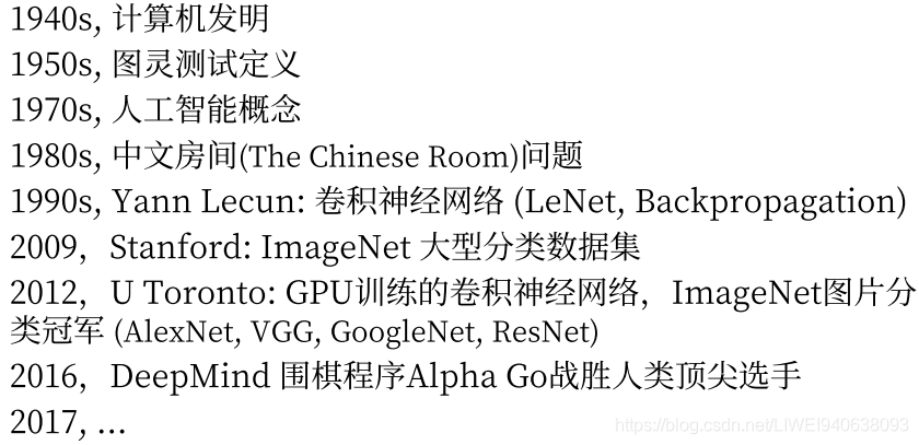

传统机器学习和深度学习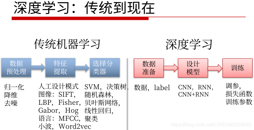

传统机器学习的数据预处理和深度学习是相通的，包括深度学习想扩大自己的训练数据集，做label，归一化，做降维，去取得更好的feature。包括clean data清洗数据集，去噪，都很类似。
传统机器学习和深度学习的主要区别在“特征提取”。
传统机器学习：
传统的任务包括图像处理，自然语言处理，特征很多时候是根据具体的任务类型由研究人员手工设计的，即Technicraft feature人手工设计的feature，会根据每个特定任务不同。
Technicraft feature好处在于很多时候可以针对具体任务进行优化，但是很多时候手工设计的模型的容量和性能都有瓶颈，所以没法通用在更多更广泛的任务上，即没法generalize到其他任务上。
后面做判别时候，比如分类和回归，SVM和随机森林已经证明是最好的两个传统分类模型，但是效果依然不如神经网络模型。在DNN发展早期，SVM和Random Forest也和神经网络结合起来一起使用，比如RCN最后一步刚开始不是用softmax，而是用SVM作分类器，而且效果比softmax更好。

传统机器学习不重要了吗

不是
如果任务很简单，数据不多，就没必要用DNN，很多时候一个简单的分类器或者一个简单的Technicraft feature，就能使任务达到很好的效果。
根据具体任务具体分析

深度学习从传统到现在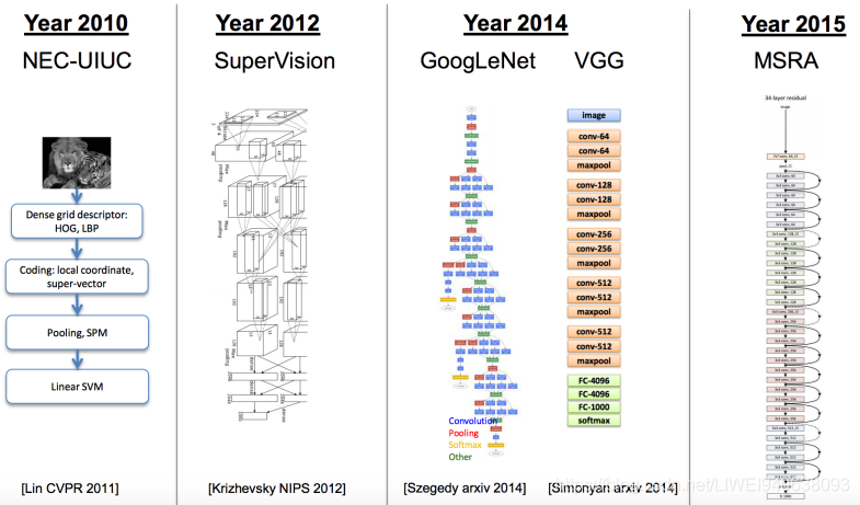

深度学习主要是在图像方面的主流模型。
几个里程碑：
1,2010NEC和UIUC一起开发的基础模型，能看到HOG,LBP，都是很传统的feature特征，最后用一个SVM做分类。
2，2012年到2015年
网络的层数和训练手段都有进步，基础的网络模型效果越来越好，造成了imagenet竞赛在2017年转到kaggle进行，全面从学术界转到了工业界，因为对学术界的价值不是很大了，它的error可以降到很小了。

近期发展的推动因素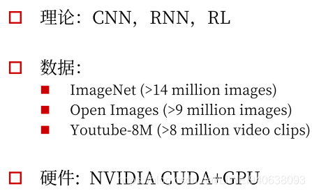

近期发展的推动因素：
理论：包括CNN,RNN,RL和其他训练手段的进步
数据：
硬件：

2.基本概念

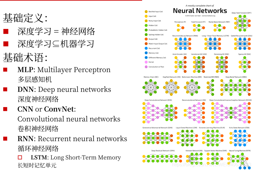
在当下深度学习概念中，深度学习的概念几乎等同于神经网络，即深度神经网络的训练和测试，运行。
深度学习基本包含于传统的机器学习定义中。传统的机器学习的优化手段和经验，数据准备和处理都可以用到深度学习中。
DNN是一个统称，各种深度神经网络(比如卷积，循环，递归)都可以用DNN来表示。

3.应用特点

图像数据是三维或四维的矩阵。
文本数据是很自然的序列数据，可以被incode成一维的向量。
语音数据也是一个线性序列的音频采样。
主要是以上三个
图像和音频结合起来可以叠加很多个frame，就是video。

自动翻译的先进项目：https://www.deepl.com/translator。 效果比google translatar更好。

优点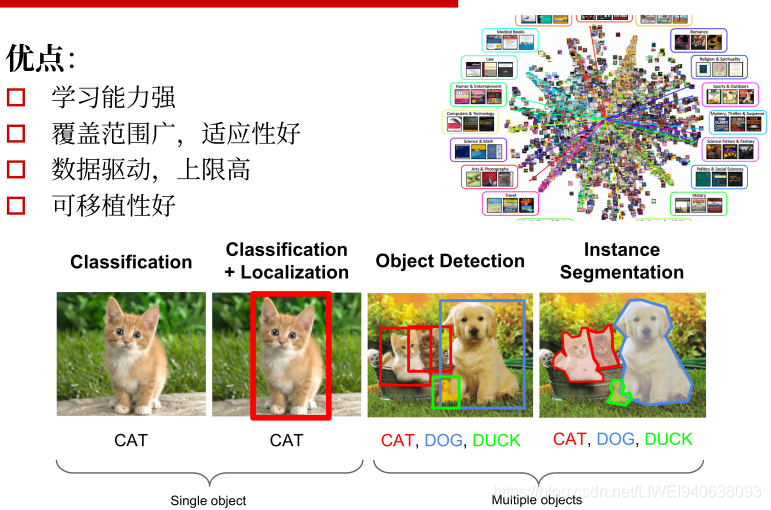

学习能力强：
深度学习就是深度神经网络的训练，层数很多，宽度很广，中间的参数记忆的容量很大，可以把神经网络当做一个高维的映射函数，理论上可以模拟任意映射函数，可以设计具体任务将需要的数据从输入空间映射到输出空间。
数据驱动，上限高：
如果设计了一个很深的模型之后，只要有足够的data，在大多数时候都会带来性能的提高。上限高就是可以进一步做online在线训练，进一步推高它的性能。
可移植性好：
深度学习框架很多。同一个数据可以设计不同神经网络，有不同应用，比如下图：
从最基础的分类:Classification给一个图片，其中有一个物体，才能分出来是猫。类别信息本身是一个标量信息，是一个scalar数据
--->Classification+Localization进一步输出它的位置信息，binary box。除类别信息:一个标量之外还有一个一维的向量。一维向量包括四个值：左上角的(x,y)，高，宽，右下角的(x,y)，这样就做了一个检测和定位。
--->Object Detection进一步做检测，分类个数超过一个，将所有相应类别都检测出来，做类别预测。
---->目前的发展趋势：Instance Segmentation(分割):不仅输出位置信息和类别(一维向量和四个number)，希望在更细化程度上标定每个pixel像素对应的物体的类别。对于每个物体，比如说狗，输出一整张mask的image，会标出每个pixel都是一个狗，这样的细化非常有用。

缺点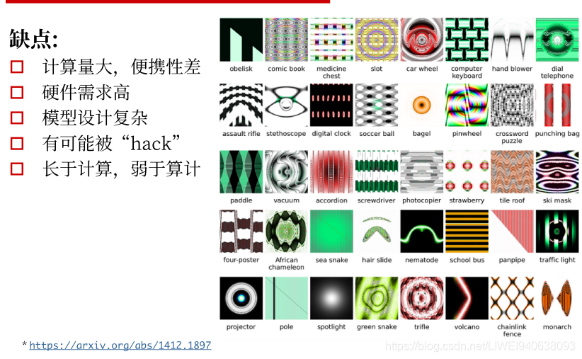

要根据自己的任务去选择模型，很多时候用传统机器学习的SVM，Random Forest就可以解决的问题，不一定就要用深度学习网络的model去用。
要用的话就要考虑计算量的问题。
有可能被hack，需要考虑训练模型的鲁棒性。

4.学习目标

二.深度学习框架与平台

1.框架比较

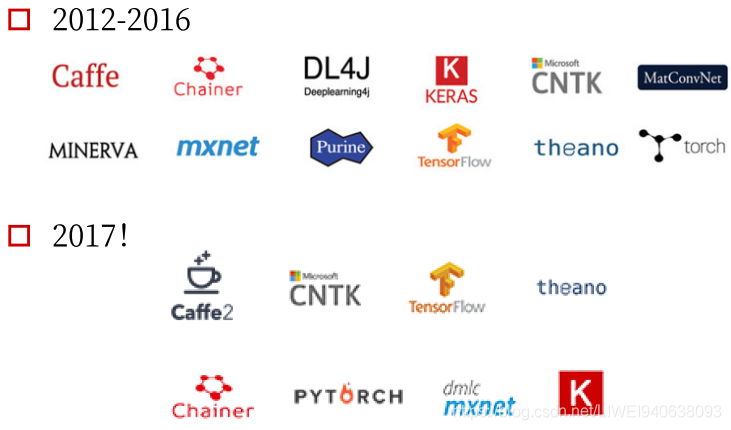
2012年AlexNET流形起来，最开始用原始的CUDA去手写自己的训练，然后去跟底层对接。
后来caffe被开发出来，在视觉领域非常流行，语言领域也不错。
在达到相应精度的条件下，caffe2所需训练时间比Tensorflow和Pytorch都更少，甚至精度会更高。

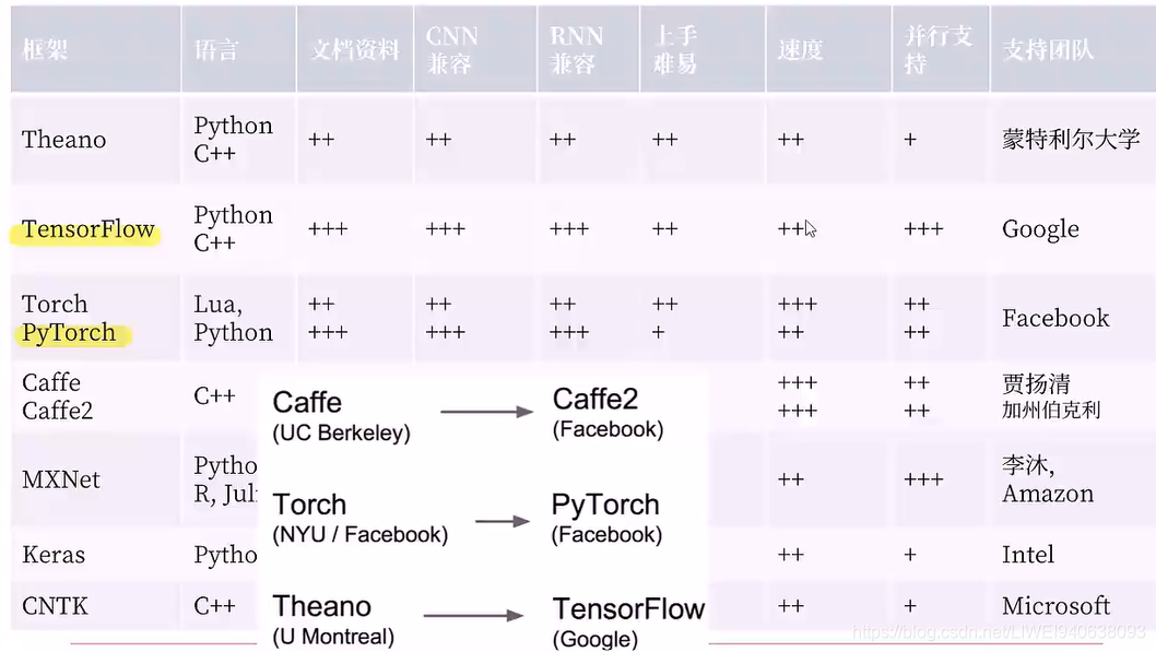
框架延续与关系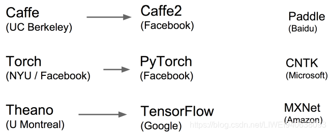

2.CPU vs GPU

cpu主要做串行运算，GPU做并行运算。
GPU做并行更好：卷积和其他神经网络的操作会用到许多矩阵运算，可以很自然地并行起来。
现在标准的跟显卡对接的两个底层框架，是CUDA和OpenCL.

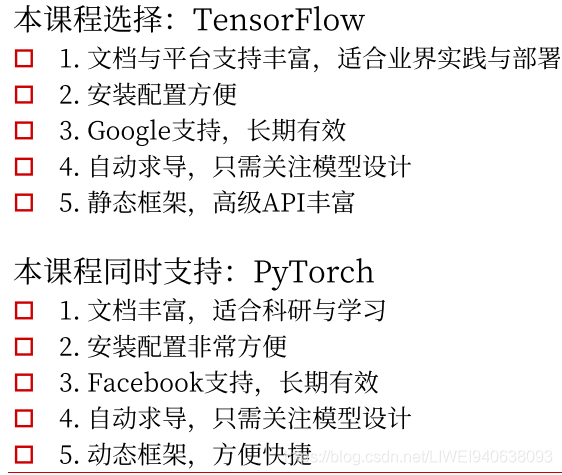
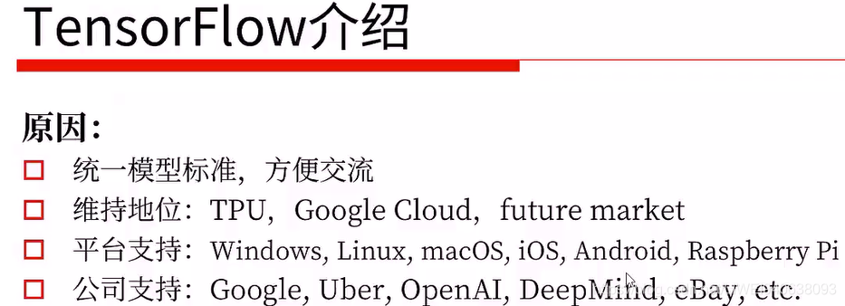
3.框架选择

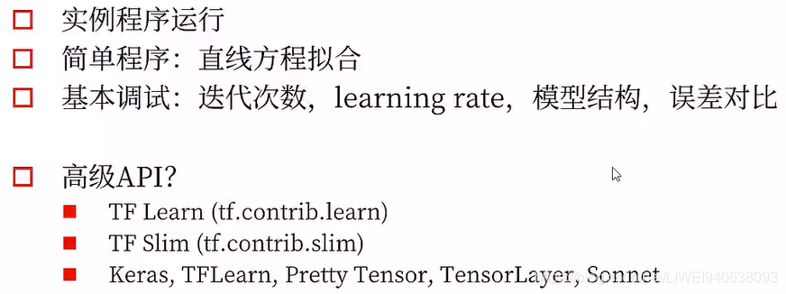
上图中，最后一行是第三方的，其中的TFLearn和上面第一行的TF Learn不是一个东西。
在这里，实例代码中尽量会用原生的TensorFlow的函数，不会去用封装的那么高级的。

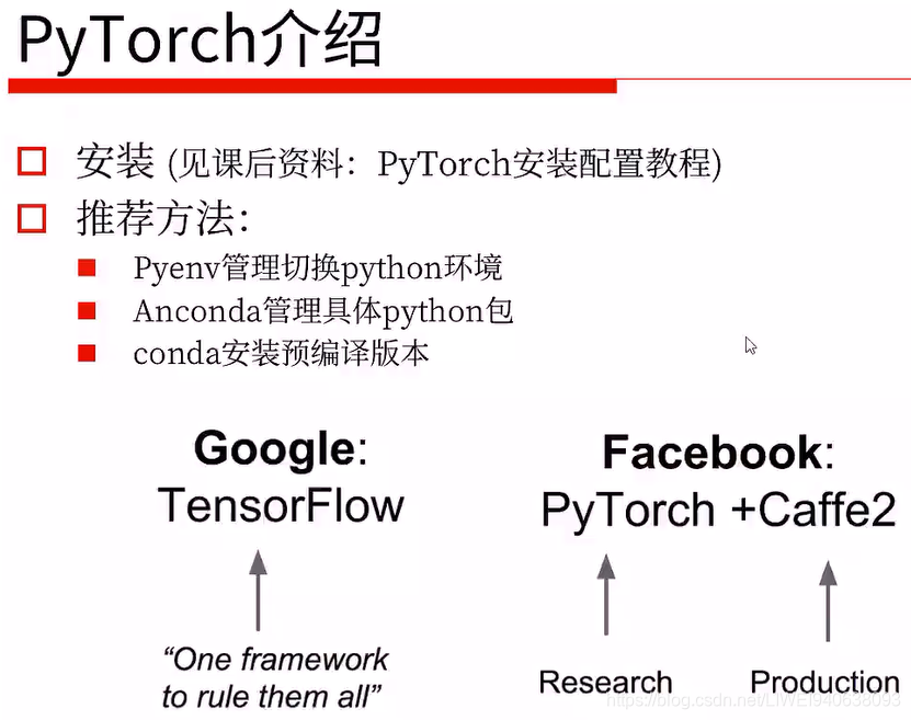
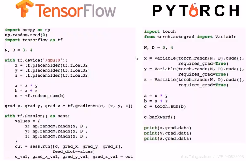
PyTorch依赖的其他包更少，很轻量，不像tensorflow。

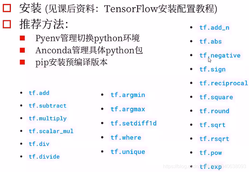
4.配置问题

Nvidia-docker
外置显卡：
外置显卡坞：雷电3外置显卡盒

三.神经网络入门

深度学习像CNN和RNN就可以把它们当做一个特征提取器feature extractor。
像素和文本都是raw feature原始特征，不可能直接去运用，要去清洗，将其转换为特征图和向量，然后再去做后面的应用。
编码的过程就相当于特征提取过程，把一个固定的图片或者一个文本映射成一个固定长度的向量，在这个向量上做解码。如果只train一个autocoder自动编码器，那前面的编码器就可以做成一个很好的特征提取器，咱们可以再调用/训练其他的解码器去对应到我们想要的任务上去。

1.基本概念

2.线性回归

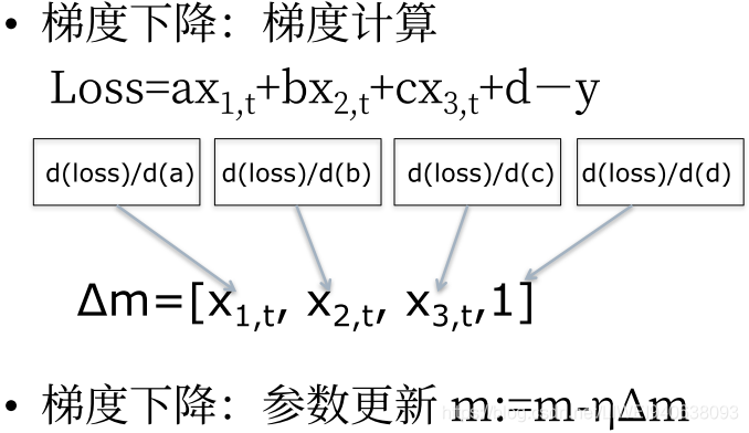
1. 优化方法：梯度下降
2. 梯度下降：梯度计算
   
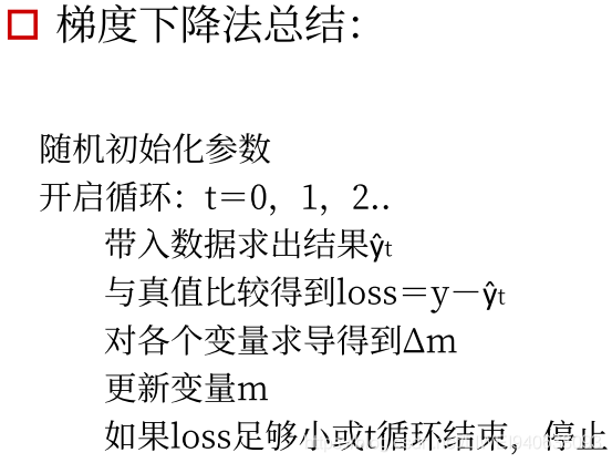
3. 梯度下降法总结
   
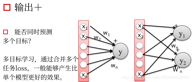
4. 输出：预测多个目标
   
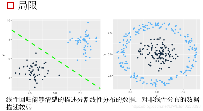
5. 局限
   

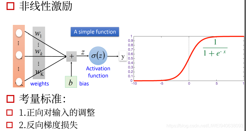
3.从线性到非线性-激励函数

4.神经元-神经网络

传统神经网络是全连接神经网络，每一个前面的unit都会和后面的unit有连接，他们的权重的size会随着unit的变化而呈指数增加，这样会产生一个问题。
比如用一个图片输入，图片本身是一个三维矩阵，如果全部用全连接层连接，到第一层feature map，每一个像素点都会和下一层feature map特征图的像素点作连接，这样传播几次权重参数会非常多。
CNN的设计特点就是考虑了局部的感知，每一个卷积核都会对一整张feature map做出响应，即空间上的平移不变形。
如何取探测不同特征？用很多卷积核，每个卷积核去关注不同的特征，最后生成很多张不同响应图图，然后叠加起来，就会生成咱们需要的特征。
在最后，才会用到全连接层。

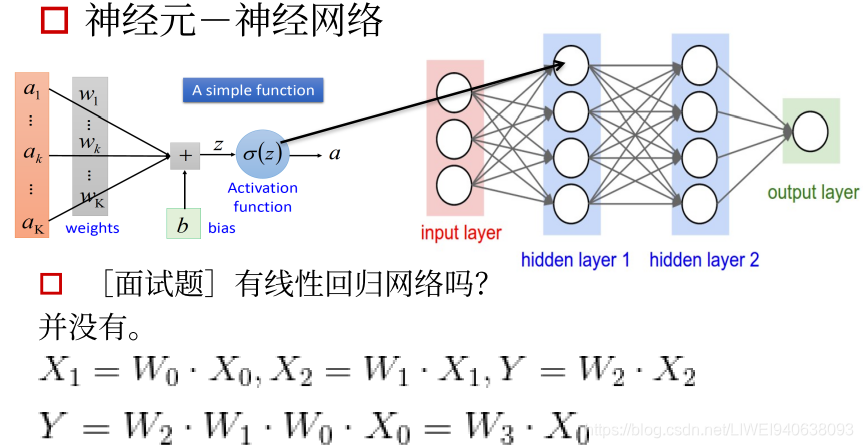
有线性回归网络吗

没有
神经网络中的激励函数必须是非线性的，如果是线性的求出来就是固定值，这样的梯度是一个定值，对优化和传播没有意义，必须用非线性的网络。

四.代码示例

tensorflow的基础操作在tensorflow中文社区都有，地址为http://www.tensorfly.cn/tfdoc/tutorials/mnist_pros.html

1.mnist_dataset_intro_tf.py

#Import MNIST导入数据集
#from tensorflow.examples.tutorials.mnist import input_data
#上面是之前的导入方法，下面为新的导入方法，tensorflow中文社区有介绍:http://www.tensorfly.cn/tfdoc/tutorials/mnist_beginners.html
#MNIST数据集的官网是Yann LeCun's website。tensorflow官网提供了下载方法，代码为https://tensorflow.googlesource.com/tensorflow/+/master/tensorflow/examples/tutorials/mnist/input_data.py
import input_data
mnist = input_data.read_data_sets("MNIST_data/", one_hot=True)

#
A next_batch function that can iterate over the whole dataset and return only the desired fraction of the dataset samples
#(in order to save memory and avoid to load the entire dataset).
# next_batch函数,迭代整个数据集并只返回所需的数据集样本的一部分 要成批fit进网络取训练，按照每张图片取训练会很慢，调整patch size尽量将显存占满为止，这样训练最快。
#batch size的大小对训练的过程和性能有影响，但是影响不大。如果只用cpu或显存特别小，调整为8/2/1都没问题，只要一个一个去训练就好了，只要确保能跑起来。
#load data
#Get the next 64 images array and labels
batch_X,batch_Y=mnist.train.next_batch(64)
#
Link:http://yann.lecun.com/exdb/mnist/

2.tensorflow_basic

# Session
Session is a class for running Tensorflow operations.A Session object encapsulate(封装/囊括)the environment in which Operation objeccts are executed,and Tensor objects are evaluated.In this tutorial,we will use a session to print out the value of tensor.Session can be used as follows:
import tensorflow as tf
a=tf.constant(100)
with tf.Session() as sess:
    print(sess.run(a))
    #syntactic sugar
    print(a.eval())
#or
sess=tf.Session()
print(sess.run(a))
#print(a,eval()) #this will print out an error.
#eval expected at least 1 arguments, got 0

#Interactive session
Interactive session is a Tensorflow session for use in interactive contexts(交互式情境),such as a shell.The only difference with a regular Session is that an Interactive session installs itself as the default session on construction.The methods Tensor.eval() and Operation.run() will use that session to run ops.This is convenient in interactive shells and Ipython notebooks,as it avoids having to pass an explicit Session object to run ops.
交互式Session在定义好之后可以将session定义为一个交互式过程，
sess=tf.InteractiveSession()
print(a.eval()) #simple usage

#Constants
We can use the help function to get an annotation(注释,说明书) about any function.Just type help(tf.constant)on the below cell and run it.It will print out(value,dtype=None,shape=None,name='Const')at the top.Value of tensor constant can be scalar(标量),matrix(矩阵) or tensor(more than 2-dimensional matrix).Also,you can get a shape of tensor by running tensor.get_shape().as_list().
. tensor.get_shape()
. tensor.get_shape().as_list()
a=tf.constant([[1,2,3],[4,5,6]],dtype=tf.float32,name='a')
print(a.eval())
print("shape:",a.get_shape(),",type:",type(a.get_shape()))
print("shape:",a.get_shape().as_list(),",type:",type(a.get_shape().as_list()))
#a.get_shape()，tensorflow本身提供的function，不是python/numpy提供的。
#numpy的很多写法包括转换是和pytorch兼容的，但是和tensorflow不兼容。
#tensorflow中定义的tensor和numpy中的array是完全不相通的，可以转换，但是numpy 的function不能直接拿过来用。

#Basic function
There are some basic functions we need to know.Those functions will be used in next tutorial 3. 基础函数：比如训练一个线性回归网络需要哪些函数
feed_forward_neural_network
.tf.argmax 
.tf.reduce_sum 
.tf.equal 
.tf.random_normal

tf.argmax
tf.argmax(input,dimension,name=None)return the index with the largest value across dimensions of a tensor.
a=tf.constant([[1,6,5],[2,3,4]])
print(a.eval())
print("argmax over axis 0")
print(tf.argmax(a,0).eval())#维度0，是列
print("argmax over axis 1")
print(tf.argmax(a,1).eval())#维度1，是行

#tf.reduce_sum
tf.reduce_sum(input_tensor,reduction_indices=None,keep_dims=False,name=None)computes the sum of elements across dimension of a tensor.Unless keep_dims is true,the rank of the tensor is reduced by 1 for each entry in reduction_indices.if keep_dims is true,the reduced dimensions are retained with length 1.If reduction_indices has no entries,all dimensions are reduced,and a tendor with a single element is teturned.

计算tensor中所有元素在所有方向所有维度上的所有的值
a=tf.constant([[1,1,1],[2,2,2]])
print(a.eval())
print("reduce_sum over entire matrix")
print(tf.reduce_sum(a).eval())
print("reduce_sum over axis 0")
print(tf.reduce_sum(a,0).eval())
print("reduce_sum over axis 0+keep dimensions")
print(tf.reduce_sum(a,0,keepdims=True).eval())
print("reduce_sum over axis 1")
print(tf.reduce_sum(a,1).eval())
print("reduce_sum over axis 1+keep dimensions")
print(tf.reduce_sum(a,1,keepdims=True).eval())
#keepdims=True,对输出结果的不同写法


#tf.equal
tf.equal(x,y,name=None)returns the truth value of (x==y) element-wise.Note taht tf.equal supports broadcasting.For more about broadcasting,please see here.
a=tf.constant([[1,0,0],[0,1,1]])
print(a.eval())
print("Equal to 1?")
print(tf.equal(a,1).eval())
print("Not equal to 1")
print(tf.not_equal(a,1).eval())
#eval,评估，鉴定


#tf.random_normal
tf.random_normal(shape,mean=0.0,stddev=1.0,dtype=tf.float32,seed=None,name=None)outputs random values from a normal distribution.
normal=tf.random_normal([3],stddev=0.1) #0维是列，1维是行
print(normal.eval())


#Variables
When we train a model,we use variables to hold  and update parameters.Variables are in-memory buffers containing tensors.They must be explicitly initialized and can be saved to disk during and after training.we can later restore saved values to exercise or analyze the model.

当训练model时，常量是常量，在跑图模型时，最基本的是需要变量，变量可以分为不同的值，根据不同的输入输出去做运算。
  .tf.Variable
  .tf.Tensor.name
  .tf.all.variables
# variable will be initialized with normal distribution
var=tf.Variable(tf.random_normal([3],stddev=0.1),name='var')
print(var.name)
tf.global_variables_initializer().run()
print(var.eval())


#tf.Tensor.name
We can call tf.Variable and give the same name my_var more than once as seen below.Note that var3.name prints out my_var_1:0 instead of my_var:0. This is because TensorFlow doesn't allow user to create variables with the same names.In this case,TensorFlow adds_1 to the original name instead of printing out an error messages.Note that you should be careful not to call tf.Variable giving same name nore than once,because it will cause a fatal problem when you save and restore the variables.
var2=tf.Variable(tf.random_normal([2,3],stddev=0.1,name='my_var'))
var3=tf.Variable(tf.random_normal([2,3],stddev=0.1,name='my_var'))
print(var2.name)
print(var3.name)


#Place holder
TensorFlow provides a placeholder operation that must be fed with data on execution.If you want to get more details about placeholder,please see here.
相当于一个容器，容器只用定义它的format就可以，具体里面是什么内容要根据具体运行的输入的值来定。结构已经定义好了，只需要用 Placeholder来占位。
x=tf.placeholder(tf.int16)
y=tf.placeholder(tf.int16)
#两个节点

add=tf.add(x,y)
mul=tf.multiply(x,y)
#两个function，映射

#launch default graph，值经过编译好的图结构
print("2+3=%d" % sess.run(add,feed_dict={x:2,y:3}))
print("3*4=%d" % sess.run(mul,feed_dict={x:3,y:4}))

3.Linear_regression_tf_online

#
A linear regression learning algorithm example using Tensorflow Library
import tensorflow as tf
import numpy
import matplotlib.pyplot as plt
rng=numpy.random
#hyperparameters超参数
learning_rate=0.01
training_epochs=100
display_step=50
#Training Data
train_X=numpy.asarray([3.3,4.4,5.5,6.71,6.93,4.168,9.779,6.182,7.59,2.167,7.042,10.791,5.313,7.997,5.654,9.27,3.1])
train_Y=numpy.asarray([1.7,2.76,2.09,3.19,1.694,1.573,3.366,2.596,2.53,1.221,2.827,3.465,1.65,2.904,2.42,2.94,1.3])
n_samples=train_X.shape[0] #0维是列，1维是行
#tf Graph Input
X=tf.placeholder("float")
Y=tf.placeholder("float")
#Set model weights
W=tf.Variable(rng.randn(),name="weight")
b=tf.Variable(rng.randn(),name="bias")
#Construct a linear model
pred=tf.add(tf.multiply(X,W),b)
#Mean squared error
cost=tf.reduce_sum(tf.pow(pred-Y,2))/(2*n_samples) #pow-power指数，sum((pred-Y)**2)/(2*n_samples)平均平方差
#Gradient descent
#定义优化器，最常用的就是梯度下降，
optimizer=tf.train.GradientDescentOptimizer(learning_rate).minimize(cost)
#以上都是在定义结构，真正的东西还没开始跑
#Initialize the variables (i.e. assign their default value)
init=tf.global_variables_initializer()
#把所有参数global_variables初始化initializer
#Start traing
with tf.Session() as sess:
    sess.run(init)
    
    #Fit all training data
    for epoch in range(100):
        for (x,y) in zip(train_X,train_Y): #zip配对
            sess.run(optimizer,feed_dict={X:x,Y:y})
            
        #Display logs per epoch step
        if (epoch+1) % display_step == 0: #每50个输出一个cost值，看跑的怎么样
            c=sess.run(cost,feed_dict={X:train_X,Y:train_Y})
            print("Epoch:",'%04d' % (epoch+1), "cost=", "{:.9f}".format(c),"W=",sess.run(W),"b=",sess.run(b))
    print("Optimization Finished!")
    training_cost=sess.run(cost,feed_dict={X:train_X,Y:train_Y})
    print("Training cost=",training_cost,"w=",sess.run(W),"b=",sess.run(b))
    
    #Graphic display
    plt.plot(train_X,train_Y,'ro',label='Original data')
    plt.plot(train_X,sess.run(W)*train_X+sess.run(b),label='Fitted line')
    plt.legend()
    plt.show()

4.pytorch-linear_regression

import torch
import torch.nn as nn
import numpy as np
import matplotlib.pyplot as plt
# Hyper-parameters
input_size = 1
output_size = 1
num_epochs = 60
learning_rate = 0.001
# Toy dataset
x_train = np.array([[3.3], [4.4], [5.5], [6.71], [6.93], [4.168], 
                    [9.779], [6.182], [7.59], [2.167], [7.042], 
                    [10.791], [5.313], [7.997], [3.1]], dtype=np.float32)

y_train = np.array([[1.7], [2.76], [2.09], [3.19], [1.694], [1.573], 
                    [3.366], [2.596], [2.53], [1.221], [2.827], 
                    [3.465], [1.65], [2.904], [1.3]], dtype=np.float32)
# Linear regression model
model = nn.Linear(input_size, output_size)
# Loss and optimizer
criterion = nn.MSELoss()
optimizer = torch.optim.SGD(model.parameters(), lr=learning_rate)  
# Train the model
for epoch in range(num_epochs):
    # Convert numpy arrays to torch tensors
    inputs = torch.from_numpy(x_train)
    targets = torch.from_numpy(y_train)

    # Forward pass
    outputs = model(inputs)
    loss = criterion(outputs, targets)
    
    # Backward and optimize
    optimizer.zero_grad()
    loss.backward()
    optimizer.step()
    
    if (epoch+1) % 5 == 0:
        print ('Epoch [{}/{}], Loss: {:.4f}'.format(epoch+1, num_epochs, loss.item()))
# Plot the graph
predicted = model(torch.from_numpy(x_train)).detach().numpy()
plt.plot(x_train, y_train, 'ro', label='Original data')
plt.plot(x_train, predicted, label='Fitted line')
plt.legend()
plt.show()

# Save the model checkpoint
torch.save(model.state_dict(), 'model.ckpt')