基于小波变换的纹理图像分割matlab仿真
目录
1.算法概述
图像分割是模式识别、计算机视觉、图像处理领域中的基础和关键。图像分割的质量直接影响到图像分析的效果。所谓图像分割是根据灰度、颜色、纹理和形状等特征把图像分成若干个特定的、互不交迭的、具有独特性质的区域。各区域的并集是整个图像,各区域的交集为空,并且这些特征在同一区域内呈现相似性,而在不同区域间呈现明显的差异性。常用的图像分割方法包括:阈值分割法、边缘检测法、区域分割法、图论分割法等。
图像分割技术近几十年来飞速发展,引起人们广泛关注。许多研究工作由原来的规则域拓展到不规则域。尤其是图论分割法成为国内外研究人员的重点研究对象之一。基于图论的图像分割是一种自上而下的全局分割方法,其主要思想是将一幅原始图像映射成一个加权、无向图,该图像中的像素对应于图中的节点,像素之间的关系对应于节点间的边,像素间的相关程度(差异性或相似性)对应于边的权重。然后在所建立的图上利用分割准则对图中的节点进行划分,进而完成对图像的分割。
ZAHN C提出一种基于图的最小生成树的图像分割方法,主要是通过将图中权值最小的边分割开来构造子图从而得到分割结果,此方法主要考虑图的局部特征,导致分割效果不理想。之后MALIK J等人提出了一种归一化分割算法,其考虑到了图像所分区域内部的自相似性,具有捕捉图像非局部特性的能力,分割效果得到很大提高,但是计算复杂度较高。FELZENSZWALB P F等人提出了一种快速算法,通过评估图的边缘值来寻找一个分段之间边界的依据,提高了分割速度,但稳定性不够。BOYKOV Y Y等人对于N维图像提出了半自动分割方法,主要考虑节点之间的边以及目标与背景之间的明显部分,然后利用图割来获取特定目标的边界,此方法扩展了处理图像的维数,但分割速度较低。GRADY L等人提出基于等周算法的全自动图像分割方法,主要通过寻找最小等周率来进行图像分割,此方法分割速度和稳定度均有了一定的提高。
由于图小波变换提供了类似于传统小波变换的多尺度分析,而且在不规则域内能够有效地检测出图像的边缘信息,因此提出一种基于图小波变换的图像分割算法。在本文中,将介绍如何利用图小波变换对定义在图上的函数进行不规则性检测;对于图像分割问题,会对图小波变换进行调整来开发一种替代工具。首先,将一幅图像映射成图。其次,利用图小波变换来获取图上节点间的小波系数。然后,对这些小波系数进行阈值处理,从而识别出图像中相应的边缘像素。
2.仿真效果预览
matlab2022a仿真


3.MATLAB部分代码预览
..................................................................
% SEGMENTATION
%   1. k-means (on sampled image)
%   2. Use centroids to classify remaining points
%   3. Classify spatially disconnected regions as separate regions
% Segmentation Step 1.
%   k-means (on sampled image)
% Compute k-means on randomly sampled points
disp('Computing k-means...');tic;
% Set number of clusters heuristically.
k = round((rDims*cDims)/(100*100)); k = max(k,8); k = min(k,16);
% Uncomment this line when MATLAB k-means unavailable
%[centroids,esq,map] = kmeanlbg(dataset,k);
[map, centroids] = kmeans(dataset, k);  % Calculate k-means (use MATLAB k-mean
disp('k-means done.');t = toc; totalt = totalt + t;
disp(['     Number of clusters: ' int2str(k)]);
disp(['Elapsed time: ' num2str(t)]);
disp(' ');
% Segmentation Step 2.
%   Use centroids to classify the remaining points
disp('Using centroids to classify all points...');tic;
globsegimage = postproc(centroids, allfeatures, rDims, cDims);   % Use centroids to classify all points
% Segmentation Step 3.
%   Classify spatially disconnected regions as separate regions
globsegimage = medfilt2(globsegimage, [3 3], 'symmetric');
globsegimage = imfill(globsegimage);
region_count = max(max(globsegimage));
count = 1; newglobsegimage = zeros(size(globsegimage));
for i = 1:region_count
    region = (globsegimage == i);
    [bw, num] = bwlabel(region);
    for j = 1:num
        newglobsegimage = newglobsegimage + count*(bw == j);
        count = count + 1;
    end
end
oldglobsegimage = globsegimage;
globsegimage = newglobsegimage;
disp('Classification done.');t = toc; totalt = totalt + t;
disp(['Elapsed time: ' num2str(t)]);
disp(' ');
% DISPLAY IMAGES
% Display segments
%figure(1), imshow(globsegimage./max(max(globsegimage)));
figure(1), imshow(label2rgb(globsegimage, 'gray'));
title('Segments');
% Calculate boundary of segments
BW = edge(globsegimage,'sobel', 0);
% Superimpose boundary on original image
iout = img;
if (depth == 1) % Gray image, so use color lines
    iout(:,:,1) = iout;
    iout(:,:,2) = iout(:,:,1);
    iout(:,:,3) = iout(:,:,1);
    iout(:,:,2) = min(iout(:,:,2) + BW, 1.0);
    iout(:,:,3) = min(iout(:,:,3) + BW, 1.0);
else            % RGB image, so use white lines
    iout(:,:,1) = min(iout(:,:,1) + BW, 1.0);
    iout(:,:,2) = min(iout(:,:,2) + BW, 1.0);
    iout(:,:,3) = min(iout(:,:,3) + BW, 1.0);
end
% Display image and segments
figure(2), imshow(iout);
title('Segmented image');
% POST PROCESSING AND AUTOMATIC SELECTION OF SOURCE AND TARGET REGIONS
%   1. Find overall textured region using Otsu's method (MATLAB graythresh)
%   2. Save each region and region boundary separately and note index of
%      textured regions
%   3. For each textured region, find all adjacent untextured regions and
%      save in adjacency matrix. Regions having a significant common border
%      are considered adjacent.
%   4. Find similarity between textured and adjacent untextured regions
%      using average gray level matching (average color matching). For each
%      textured region, drop those adjacent regions which don't match in
%      gray level.
disp('Post-processing and automatically selecting source and target regions...');tic;
% POSTPROC Step 1
threshold = graythresh(rescalegray(textures));
bwtexture = textures > threshold;
tex_edges = edge(bwtexture, 'sobel', 0);
figure(3),
if depth == 1
    imshow(min(img + tex_edges, 1));
else
    imshow(min(img + cat(3, tex_edges, tex_edges, tex_edges), 1));
end
title('Textured regions');
% POSTPROC Step 2
% Save each region in a dimension
% Save each region boundary in a dimension
% For each region which can be classified as a textured region store index
region_count = max(max(globsegimage));
number_tex_regions = 1; tex_list = [];
for region_number = 1:region_count
    bwregion = (globsegimage == region_number);

    regions(:,:,region_number) = bwregion; % Save all regions
    region_boundaries(:,:,region_number) = edge(bwregion, 'sobel', 0);
    if ( (sum(sum(bwregion.*bwtexture))/sum(sum(bwregion)) > 0.75) && sum(sum(bwregion)) > (32*32) )
        tex_list = [tex_list region_number];
        number_tex_regions = number_tex_regions + 1;
    end
end
number_tex_regions = number_tex_regions - 1;
% POSTPROC Step 3
% Find texture region adjacency and create an adjacency matrix
for i = 1:size(tex_list, 2)
    for j = 1:region_count
        if (tex_list(i) ~= j)
            boundary_overlap = sum(sum( region_boundaries(:,:,tex_list(i)).*region_boundaries(:,:,j) ));
            boundary_total_length = sum(sum( region_boundaries(:,:,tex_list(i)))) + sum(sum(region_boundaries(:,:,j)));
            if (boundary_overlap/boundary_total_length > 0) % If overlap is at least 20% of total boundary length
                region_adjacency(i,j) = boundary_overlap;     % accept it as a boundary
            end
        end
    end
end
% EXPERIMENTAL
region_adj_hard_coded = (region_adjacency - 0.2*repmat(mean(region_adjacency,2), [1 size(region_adjacency,2)])) > 0;
% Copy adjacency into another variable and remove all references to
% textured regions from the adjacency matrix.
region_output = region_adj_hard_coded;
for tex_count = 1:size(tex_list, 2)
    region_output(:,tex_list(tex_count)) = 0;
end
% POSTPROC Step 4
% Find similarity between textured and adjacent untextured regions
% (This could be changed to a chi-squared distance between histograms of
%  textLP and adjacent by commenting out required code, and uncommenting
%  other code, as directed in the source)
% For all textured regions find and save average brightness
for tex_count = 1:size(tex_list, 2)
    if depth == 1
        tex_avg_bright(tex_count) = sum(sum(regions(:,:,tex_list(tex_count)).*lowpassimage)) ...
                         / sum(sum(regions(:,:,tex_list(tex_count))));
        % Comment previous and uncomment next line(s) to use histogram
        % processing
        %tex_hist{tex_count} = histproc(regions(:,:,tex_list(tex_count)), lowpassimage);
    else
        tex_avg_bright(1,tex_count) = sum(sum(regions(:,:,tex_list(tex_count)).*lowpassimage(:,:,1))) ...
                                / sum(sum(regions(:,:,tex_list(tex_count))));
        tex_avg_bright(2,tex_count) = sum(sum(regions(:,:,tex_list(tex_count)).*lowpassimage(:,:,2))) ...
                                / sum(sum(regions(:,:,tex_list(tex_count))));
        tex_avg_bright(3,tex_count) = sum(sum(regions(:,:,tex_list(tex_count)).*lowpassimage(:,:,3))) ...
                                / sum(sum(regions(:,:,tex_list(tex_count))));
        % Comment previous and uncomment next line(s) to use histogram
        % processing
        % tex_hist{tex_count} = histproc(regions(:,:,tex_list(tex_count)), lowpassimage);
    end
end
% For all textured regions, consider each non-textured region and update
% adjacency matrix. Keep the relationship if gray levels (colors) are similar and
% drop if the gray levels (colors) don't match.
for tex_count = 1:size(tex_list, 2) % For all textured regions
    for adj_reg_count = 1:size(region_adj_hard_coded, 2)
        if (region_adj_hard_coded(tex_count, adj_reg_count) > 0)
            if depth == 1
                region_avg_bright = sum(sum(regions(:,:,adj_reg_count).*lowpassimage)) ...
                                    / sum(sum(regions(:,:,adj_reg_count)));
                % Comment previous and uncomment next line(s) to use histogram
                % processing
                % region_hist = histproc(regions(:,:,adj_reg_count), lowpassimage);
            else
                region_avg_bright(1) = sum(sum(regions(:,:,adj_reg_count).*lowpassimage(:,:,1))) ...
                                    / sum(sum(regions(:,:,adj_reg_count)));
                region_avg_bright(2) = sum(sum(regions(:,:,adj_reg_count).*lowpassimage(:,:,2))) ...
                                    / sum(sum(regions(:,:,adj_reg_count)));
                region_avg_bright(3) = sum(sum(regions(:,:,adj_reg_count).*lowpassimage(:,:,3))) ...
                                    / sum(sum(regions(:,:,adj_reg_count)));
                % Comment previous and uncomment next line(s) to use histogram
                % processing
                % region_hist = histproc(regions(:,:,adj_reg_count), lowpassimage);
            end

            if depth == 1
                if abs(tex_avg_bright(tex_count) - region_avg_bright) > 0.2 % Highly similar
                    region_output(tex_count, adj_reg_count) = 0;
                end
                % Comment previous and uncomment next line(s) to use histogram
                % processing
%                 if chisq(tex_hist{tex_count}, region_hist) > 0.4
%                     chisq(tex_hist{tex_count}, region_hist)
%                     region_output(tex_count, adj_reg_count) = 0;
%                 end
            else
                if mean(abs(tex_avg_bright(:,tex_count) - region_avg_bright')) > 0.2
                    region_output(tex_count, adj_reg_count) = 0;
                end
                % Comment previous and uncomment next line(s) to use histogram
                % processing
%                 thist = tex_hist{tex_count};
%                 chisq(thist(:,1),region_hist(:,1))
%                 chisq(thist(:,2),region_hist(:,2))
%                 chisq(thist(:,3),region_hist(:,3))
%                 t = 0.9;
%                 if (chisq(thist(:,1),region_hist(:,1)) > t) || ...
%                    (chisq(thist(:,2),region_hist(:,2)) > t) || ...
%                    (chisq(thist(:,3),region_hist(:,3)) > t)
%                     region_output(tex_count, adj_reg_count) = 0;
%                 end
            end
        end
    end
end
disp('Post-processing done.'); t = toc; totalt = totalt + t;
disp(['Elapsed time: ' num2str(t)]);
disp(' ');
disp(['Total time elapsed: ' int2str(floor(totalt/60)) ' minutes ' int2str(mod(totalt,60)) ' seconds.']);
% DISPLAY IMAGES
% Display source and target regions.
if depth == 1
    imgs = zeros([rDims cDims size(tex_list,2)]);
    for tex_count = 1:size(tex_list, 2)
        if (sum(region_output(tex_count,:) > 0)) % If we have target patches
            imgs(:,:,tex_count) = regions(:,:,tex_list(tex_count)).*img; % Save that source patch
            for i = 1:size(region_output, 2) % For each region
                if (region_output(tex_count, i) > 0)    % which is connected to that source patch
                    imgs(:,:,tex_count) = imgs(:,:,tex_count) + 0.5*regions(:,:,i).*img; % Save the target patch
                end
            end
            figure, imshow(min(imgs(:,:,tex_count) + BW, 1));
            ggg{tex_count} = min(imgs(:,:,tex_count) + BW, 1);
            title('Potential source and target regions');
        end
    end
else % depth == 3
    count = 1;
    for tex_count = 1:size(tex_list, 2)
        if (sum(region_output(tex_count,:) > 0)) % If we have target patches
            tmp(:,:,1) = regions(:,:,tex_list(tex_count)).*img(:,:,1);
            tmp(:,:,2) = regions(:,:,tex_list(tex_count)).*img(:,:,2);
            tmp(:,:,3) = regions(:,:,tex_list(tex_count)).*img(:,:,3);
            imgs{count} = tmp;
            for i = 1:size(region_output, 2) % For each region
                if (region_output(tex_count, i) > 0)    % which is connected to that source patch
                    tmp(:,:,1) = 0.5*regions(:,:,i).*img(:,:,1);
                    tmp(:,:,2) = 0.5*regions(:,:,i).*img(:,:,2);
                    tmp(:,:,3) = 0.5*regions(:,:,i).*img(:,:,3);
                    imgs{count} = imgs{count} + tmp;
                end
            end
            figure, imshow(min(imgs{count} + cat(3,BW,BW,BW), 1));
            ggg{count} = min(imgs{count} + cat(3,BW,BW,BW), 1);
            title('Potential source and target regions');
            count = count+1;
        end
    end
end
A-012
4.完整MATLAB程序
V

CSDN联合极客时间,共同打造面向开发者的精品内容学习社区,助力成长!
更多推荐

 0
0 0
0- 0


 已为社区贡献4条内容

所有评论(0)