deeplearning.ai笔记
课程在网易云课堂上免费观看,作业题如下:加粗为答案。神经网络和深度学习网址第一周 深度学习概论第二周 Logistic RegressionLogistic回归公式推导样本个数 mmm, 训练样本个数 mtrainmtrainm_{train}, 同理 mtestmtestm_{test},mvalidmvalidm_{valid}单个样本...
课程在网易云课堂上免费观看,作业题如下:加粗为答案。
神经网络和深度学习
第一周 深度学习概论
第二周 Logistic Regression
Logistic回归公式推导
样本个数 m m <script type="math/tex" id="MathJax-Element-1">m</script>, 训练样本个数 <script type="math/tex" id="MathJax-Element-2">m_{train}</script>, 同理 mtest m t e s t <script type="math/tex" id="MathJax-Element-3">m_{test}</script>, mvalid m v a l i d <script type="math/tex" id="MathJax-Element-4">m_{valid}</script>
单个样本
forward propagate
input x的shape为 (nx,1) ( n x , 1 ) <script type="math/tex" id="MathJax-Element-5">(n_x, 1)</script>,label y的shape为 (1,1) ( 1 , 1 ) <script type="math/tex" id="MathJax-Element-6">(1, 1)</script>
weights w的shape为 (nx,1) ( n x , 1 ) <script type="math/tex" id="MathJax-Element-8">(n_x, 1)</script>,biases b的shape为 (1,1) ( 1 , 1 ) <script type="math/tex" id="MathJax-Element-9">(1, 1)</script>
z的shape为 (1,1) ( 1 , 1 ) <script type="math/tex" id="MathJax-Element-11">(1, 1)</script>
output y^ y ^ <script type="math/tex" id="MathJax-Element-13">\hat{y}</script>的shape为 (1,1) ( 1 , 1 ) <script type="math/tex" id="MathJax-Element-14">(1, 1)</script>
损失函数 l(y^,y) l ( y ^ , y ) <script type="math/tex" id="MathJax-Element-16">l(\hat{y},y)</script>的shape为 (1,1) ( 1 , 1 ) <script type="math/tex" id="MathJax-Element-17">(1, 1)</script>
backward propagate
损失函数对 y^ y ^ <script type="math/tex" id="MathJax-Element-19">\hat{y}</script>和 a a <script type="math/tex" id="MathJax-Element-20">a</script>的偏导
损失函数对 z z <script type="math/tex" id="MathJax-Element-22">z</script>的偏导
损失函数对 dw d w <script type="math/tex" id="MathJax-Element-24">d_w</script>的偏导
$$
\begin {aligned}
d_{w_1} &= \frac{\partial l}{\partial z} \frac{\partial z}{\partial w_1} \
&= (a-y) * \frac{\partial z}{\partial w_1}(w_1x_1+\cdots+w_nx_n+b) \
&= x_1 * (a-y) \
d_w &= \left[
\right] \
&=
\left[
\right] (a-y)
\end {aligned}
$$
损失函数对 db d b <script type="math/tex" id="MathJax-Element-27">d_b</script>的偏导
根据导数对梯度进行更新的计算公式
m个样本
forward propagate
input X的shape为 (nx,m) ( n x , m ) <script type="math/tex" id="MathJax-Element-30">(n_x, m)</script>,label Y的shape为 (1,m) ( 1 , m ) <script type="math/tex" id="MathJax-Element-31">(1, m)</script>
weights w的shape为 (nx,1) ( n x , 1 ) <script type="math/tex" id="MathJax-Element-33">(n_x, 1)</script>,biases b的shape为 (1,1) ( 1 , 1 ) <script type="math/tex" id="MathJax-Element-34">(1, 1)</script> 和单个样本一样
z的shape为 (1,m) ( 1 , m ) <script type="math/tex" id="MathJax-Element-36">(1, m)</script>
output Y^ Y ^ <script type="math/tex" id="MathJax-Element-38">\hat{Y}</script>的shape为 (1,m) ( 1 , m ) <script type="math/tex" id="MathJax-Element-39">(1, m)</script>
损失函数 J(w,b) J ( w , b ) <script type="math/tex" id="MathJax-Element-41">J(w,b)</script>的shape为 (1,1) ( 1 , 1 ) <script type="math/tex" id="MathJax-Element-42">(1, 1)</script>
backward propagate
损失函数对 dZ d Z <script type="math/tex" id="MathJax-Element-44">d_Z</script>的偏导
$$
\begin {aligned}
d_{z^{(1)}} &= \frac{\partial J(w,b)}{\partial a^{(1)}} \frac{\partial a^{(1)}}{\partial z^{(1)}} \
&= -\frac{1}{m} \frac{\partial l(a^{(1)}, y^{(1)})}{\partial a^{(1)}} \frac{\partial a^{(1)}}{\partial z^{(1)}} \
&= -\frac{1}{m} d_{z^{(1)}} \
&= a^{(1)}-y^{(1)} \
d_Z &=
\left[
\begin {matrix}
d_{z^{(1)}} & \cdots & d_{z^{(m)}}
\end {matrix}
\right] \
&=
\left[
\begin {matrix}
a^{(1)}-y^{(1)} & \cdots & a^{(m)}-y^{(m)}
\end {matrix}
\right]
\end {aligned}
$$
损失函数对 dw1 d w 1 <script type="math/tex" id="MathJax-Element-45">d_{w_1}</script>的偏导
损失函数对 dW d W <script type="math/tex" id="MathJax-Element-47">d_W</script>的偏导
损失函数对 db d b <script type="math/tex" id="MathJax-Element-49">d_b</script>的偏导
根据导数对梯度进行更新的计算公式
第三周 浅层神经网络
公式推导
右上角[]表示层数,右上角()表示样本数
a[0]=X a [ 0 ] = X <script type="math/tex" id="MathJax-Element-52">a^{[0]}=X</script> 第0层为输入层
a[1]2 a 2 [ 1 ] <script type="math/tex" id="MathJax-Element-53">a^{[1]}_2</script> 表示第一层中第二个神经元
g(1) g ( 1 ) <script type="math/tex" id="MathJax-Element-54">g(1)</script>为第一层网络的激活函数
forward propagate
输入X的shape为 (n[0],m) ( n [ 0 ] , m ) <script type="math/tex" id="MathJax-Element-55">(n^{[0]},m)</script>, Y的shape为 (1,m) ( 1 , m ) <script type="math/tex" id="MathJax-Element-56">(1,m)</script>
$$
X =
\left[
\begin {matrix}
x^{(1)}_1 & \cdots & x^{(m)}_1 \
\vdots & \ddots & \vdots \
x^{(1)}_n & \cdots & x^{(m)}_n
\end {matrix}
\right]
\quad
Y =
\left[
\begin {matrix}
y^{(1)} & \cdots & y^{(m)}
\end {matrix}
\right]
$$
权重矩阵 W[1] W [ 1 ] <script type="math/tex" id="MathJax-Element-57">W^{[1]}</script>的shape为 (n[1],n[0]) ( n [ 1 ] , n [ 0 ] ) <script type="math/tex" id="MathJax-Element-58">(n^{[1]}, n^{[0]})</script>, 偏置 b[1] b [ 1 ] <script type="math/tex" id="MathJax-Element-59">b^{[1]}</script>的shape为 (n[1],1) ( n [ 1 ] , 1 ) <script type="math/tex" id="MathJax-Element-60">(n^{[1]}, 1)</script>
$$
\begin {aligned}
W^{[1]} &=
\left[
\begin {matrix}
w_{1,1} & \cdots & w_{1,n^{[0]}} \
\vdots & \ddots & \vdots \
w_{n^{[1]},1} & \cdots & w_{n^{[1]},n^{[0]}}
\end {matrix}
\right] \
b^{[1]} &=
\left[
\begin {matrix}
b_{1} \
\vdots \
b_{n^{[1]}}
\end {matrix}
\right]
\end {aligned}
$$
第一层神经元 Z[1] Z [ 1 ] <script type="math/tex" id="MathJax-Element-61">Z^{[1]}</script>、 A[1] A [ 1 ] <script type="math/tex" id="MathJax-Element-62">A^{[1]}</script>的shape为 (n[1],m) ( n [ 1 ] , m ) <script type="math/tex" id="MathJax-Element-63">(n^{[1]},m)</script>
$$
\begin {aligned}
Z^{[1]}
&= W^{[1]} X + b^{[1]} \
&=
\left[
\begin {matrix}
w_{1,1} & \cdots & w_{1,n^{[0]}} \
\vdots & \ddots & \vdots \
w_{n^{[1]},1} & \cdots & w_{n^{[1]},n^{[0]}}
\end {matrix}
\right]
\left[
\begin {matrix}
x^{(1)}_1 & \cdots & x^{(m)}_1 \
\vdots & \ddots & \vdots \
x^{(1)}_n & \cdots & x^{(m)}_n
\end {matrix}
\right]
+
\left[
\begin {matrix}
b_{1} \
\vdots \
b_{n^{[1]}}
\end {matrix}
\right] \
&=
\left[
\begin {matrix}
z_{1}^{[1] (1)} & \cdots & z_{1}^{[1] (m)} \
\vdots & \ddots & \vdots \
z_{n^{[1]}}^{[1] (1)} & \cdots & z_{n^{[1]}}^{[1] (m)}
\end {matrix}
\right] \
A^{[1]} &=
g(1)(Z^{[1]})
\end {aligned}
$$
权重矩阵 W[2] W [ 2 ] <script type="math/tex" id="MathJax-Element-64">W^{[2]}</script>的shape为 (n[2],n[1]) ( n [ 2 ] , n [ 1 ] ) <script type="math/tex" id="MathJax-Element-65">(n^{[2]}, n^{[1]})</script>, 偏置 b[2] b [ 2 ] <script type="math/tex" id="MathJax-Element-66">b^{[2]}</script>的shape为 (n[2],1) ( n [ 2 ] , 1 ) <script type="math/tex" id="MathJax-Element-67">(n^{[2]}, 1)</script>
$$
\begin {aligned}
W^{[2]} &=
\left[
\begin {matrix}
w_{1,1} & \cdots & w_{1,n^{[1]}} \
\vdots & \ddots & \vdots \
w_{n^{[2]},1} & \cdots & w_{n^{[2]},n^{[1]}}
\end {matrix}
\right] \
b^{[2]} &=
\left[
\begin {matrix}
b_{1} \
\vdots \
b_{n^{[2]}}
\end {matrix}
\right]
\end {aligned}
$$
第二层神经元 Z[2] Z [ 2 ] <script type="math/tex" id="MathJax-Element-68">Z^{[2]}</script>、 A[2] A [ 2 ] <script type="math/tex" id="MathJax-Element-69">A^{[2]}</script>的shape为 (n[2],m) ( n [ 2 ] , m ) <script type="math/tex" id="MathJax-Element-70">(n^{[2]},m)</script>
$$
\begin {aligned}
Z^{[2]}
&= W^{[2]} A^{[1]} + b^{[2]} \
&=
\left[
\begin {matrix}
z_{1}^{[2] (1)} & \cdots & z_{1}^{[2] (m)} \
\vdots & \ddots & \vdots \
z_{n^{[1]}}^{[2] (1)} & \cdots & z_{n^{[1]}}^{[2] (m)}
\end {matrix}
\right] \
A^{[2]} &=
g(2)(Z^{[2]})
\end {aligned}
$$
损失函数为
backward propagate
当 g(2) g ( 2 ) <script type="math/tex" id="MathJax-Element-72">g(2)</script>为sigmoid函数时
四种激活函数及其导数
第四周 深层神经网络
公式
其中, l l <script type="math/tex" id="MathJax-Element-83">l</script>为层数,总层数为 <script type="math/tex" id="MathJax-Element-84">L</script>, l=0 l = 0 <script type="math/tex" id="MathJax-Element-85">l=0</script>表示输入层 X X <script type="math/tex" id="MathJax-Element-86">X</script>, <script type="math/tex" id="MathJax-Element-87">l=L</script>表示输出层
W[l] W [ l ] <script type="math/tex" id="MathJax-Element-88">W^{[l]}</script>的shape为 (n[l],n[l−1]) ( n [ l ] , n [ l − 1 ] ) <script type="math/tex" id="MathJax-Element-89">(n^{[l]}, n^{[l-1]})</script>
Z[l] Z [ l ] <script type="math/tex" id="MathJax-Element-90">Z^{[l]}</script> A[l] A [ l ] <script type="math/tex" id="MathJax-Element-91">A^{[l]}</script>的shape为 (n[l],m) ( n [ l ] , m ) <script type="math/tex" id="MathJax-Element-92">(n^{[l]}, m)</script>
b[l] b [ l ] <script type="math/tex" id="MathJax-Element-93">b^{[l]}</script>的shape为 (n[l],1) ( n [ l ] , 1 ) <script type="math/tex" id="MathJax-Element-94">(n^{[l]}, 1)</script>
改善深层神经网络:超参数调试、正则化以及优化
第一周 深度学习的实用层面
训练/开发/测试集
对于100万以上数据 train 98% dev/valid 1% test 1%
偏差bias/方差variance
训练集上的高偏差?
加深网络、换网络模型
验证集上的高方差?
更多的数据、正则化
正则化-L2
L2正则化, J(w,b)=1m∑mi=1l(a(i),y(i))+λ2m||w||2 J ( w , b ) = 1 m ∑ m i = 1 l ( a ( i ) , y ( i ) ) + λ 2 m | | w | | 2 <script type="math/tex" id="MathJax-Element-96">J(w,b)=\frac{1}{m} \sum{m \atop i=1}{l(a^{(i)},y^{(i)})}+\frac{\lambda}{2m}||w||^2</script>
λ λ <script type="math/tex" id="MathJax-Element-97">\lambda</script>表示正则化参数,python编程时用lambd表示。
||w||2 | | w | | 2 <script type="math/tex" id="MathJax-Element-98">||w||^2</script>表示权重矩阵中所有权重值的平方和。
对上式子进行求导,会得到 dW[l]=(frombackpropa)+λmW[l] d W [ l ] = ( f r o m b a c k p r o p a ) + λ m W [ l ] <script type="math/tex" id="MathJax-Element-99">\mathrm{d}W^{[l]}=(from backpropa)+\frac{\lambda}{m}W^{[l]}</script>
权重更新公式为 W[l]=W[l]−dW[l]=(1−aλm)W[l]−a(frombackpropa) W [ l ] = W [ l ] − d W [ l ] = ( 1 − a λ m ) W [ l ] − a ( f r o m b a c k p r o p a ) <script type="math/tex" id="MathJax-Element-100">W^{[l]}=W^{[l]}-\mathrm{d}W^{[l]}=(1-\frac{a\lambda}{m})W^{[l]}-a(from backpropa)</script>
权重会不断的下降,所以也称之为权重衰减。weight decay
λ λ <script type="math/tex" id="MathJax-Element-101">\lambda</script>越大, Z Z <script type="math/tex" id="MathJax-Element-102">Z</script>越小,tanh或者sigmoid激活函数越接近于线性,整个神经网络会向线性方向发展,这样就会避免过拟合。
正则化-dropout
Inverted dropout
d3 = np.random.randn(a3.shape[0], a3.shape[1]) < keep-prob
a3 = np.multiply(d3, a3)
a3 /= keep-prob
其他正则化方法
数据扩增,包含翻转、旋转、缩放、扭曲等。
early stopping,在中间点停止迭代过程。
输入归一化
将输入归一化为正太分布
使得代价函数更加圆滑,梯度更加合理
梯度消失和梯度爆炸
vanishing/exploding gradients
W^10000,W<1,消失 >1,爆炸
权重初始化
机器学习的模型(e.g. logistic regression, RBM)中为什么加入bias?
对于relu神经元, W[l]=np.random.randn(shape)∗np.sqrt(an[l−1]) W [ l ] = n p . r a n d o m . r a n d n ( s h a p e ) ∗ n p . s q r t ( a n [ l − 1 ] ) <script type="math/tex" id="MathJax-Element-104">W^{[l]}=np.random.randn(shape)*np.sqrt(\frac{a}{n^{[l-1]}})</script>
对于tanh神经元,会乘以 np.sqrt(1n[l−1]) n p . s q r t ( 1 n [ l − 1 ] ) <script type="math/tex" id="MathJax-Element-105">np.sqrt(\frac{1}{n^{[l-1]}})</script>或者 np.sqrt(2n[l−1]+n[l]) n p . s q r t ( 2 n [ l − 1 ] + n [ l ] ) <script type="math/tex" id="MathJax-Element-106">np.sqrt(\frac{2}{n^{[l-1]}+n^{[l]}})</script>,被称之为Xavierc初始化。
梯度检查
grad check
不要在训练中使用,仅仅debug
如果检查失败,检查bug
不要忘记正则化
不要使用dropout
防止过拟合的方法
- 降低模型复杂度
- 扩充样本,数据增强
- 随机裁剪
- 随机加光照
- 随机左右翻转
- early stopping
- dropout
- weight penality L1&L2
数据集少怎么办
- 图像平移
- 图像旋转
- 图像镜像
- 图像亮度变化
- 裁剪
- 缩放
- 图像模糊
第二周 优化算法
Mini-batch
64 128 512 1024
不会稳定的想最小值发展,不会收敛
动量梯度下降
指数加权平均,滑动平均模型
包含两个超参数:学习率 α α <script type="math/tex" id="MathJax-Element-108">\alpha</script>和滑动衰减率 β β <script type="math/tex" id="MathJax-Element-109">\beta</script>, β β <script type="math/tex" id="MathJax-Element-110">\beta</script>一般取0.9或者0.99,越多模型越稳定。
Momentum是为了对冲mini-batch带来的抖动。
RMSprop
$$
\begin {aligned}
S_{\mathrm{d}W} &= \beta S_{\mathrm{d}W} + (1-\beta)(\mathrm{d}W)^2 \
S_{\mathrm{d}b} &= \beta S_{\mathrm{d}b} + (1-\beta)(\mathrm{d}b)^2 \
W &= W - \alpha \frac{\mathrm{d}W}{\sqrt{S_{\mathrm{d}W}}+\varepsilon} \
b &= b - \alpha \frac{\mathrm{d}b}{\sqrt{S_{\mathrm{d}b}}+\varepsilon} \
\end {aligned}
$
ε ε <script type="math/tex" id="MathJax-Element-111">\varepsilon</script>为了阻止除以极小值,一般取e-8
RMSprop是为了对hyper-parameter进行归一。直观理解是将摆动大的梯度进行缩小。
Adam优化算法
Adaptive Moment Estimation 结合了动量和RMSprop
mini-batch中计算出每次迭代过程 t t <script type="math/tex" id="MathJax-Element-112">t</script>的 <script type="math/tex" id="MathJax-Element-113">\mathrm{d}W</script>和 db d b <script type="math/tex" id="MathJax-Element-114">\mathrm{d}b</script>后,Adam优化算法公式如下:
第三行和第四行公式为偏差修正
- α α <script type="math/tex" id="MathJax-Element-116">\alpha</script>:全局学习率
- β1 β 1 <script type="math/tex" id="MathJax-Element-117">\beta_1</script>:默认0.9
- β2 β 2 <script type="math/tex" id="MathJax-Element-118">\beta_2</script>:默认0.999
- ε ε <script type="math/tex" id="MathJax-Element-119">\varepsilon</script>:默认 10−8 10 − 8 <script type="math/tex" id="MathJax-Element-120">10^{-8}</script>
学习率衰减
学习率随着时间而慢慢变小,初始学习率,衰减率
局部最优问题
鞍点saddle point—-损失函数中的0梯度点
平滑段使得训练变慢
第三周 超参数调试、Batch正则化和程序框架
超参
按重要程度排名
- 学习率 α α <script type="math/tex" id="MathJax-Element-121">\alpha</script>——最重要
- 对对数轴上均匀取值 [10a,10b] [ 10 a , 10 b ] <script type="math/tex" id="MathJax-Element-122">[10^a,10^b]</script>,比如a,b的取值为[-4,-1]
- 隐藏层神经元个数
#hidden units——第二重要 - mini-batch size——第二重要
- moment beta——第二重要
- 0.9意味着取过去10个数字的平均值,0.999以为着取过去1000个数字的平均值
- 针对 1−β 1 − β <script type="math/tex" id="MathJax-Element-123">1-\beta</script>对对数轴上均匀取值 [10a,10b] [ 10 a , 10 b ] <script type="math/tex" id="MathJax-Element-124">[10^a,10^b]</script>,比如a,b的取值为[-3,-1]
- 隐藏层数——第三重要
- 学习率衰减值——第三重要
- Adam算法中的 β1,β2,ε β 1 , β 2 , ε <script type="math/tex" id="MathJax-Element-125">\beta_1,\beta_2,\varepsilon</script>,一般取默认值——不重要
超参搜索
- 随机选择超参组合
- 在各个参数的合理范围内随机取值
- 有助于发现潜在的最优值
- 由粗到精的搜索
Batch归一化
将每一层的Z[l]归一化,在激活之前。可以加快训练速度
Softmax层
激活函数公式
Softmax相比于Hardmax
Softmax: [0.1,0.2,0.7]T [ 0.1 , 0.2 , 0.7 ] T <script type="math/tex" id="MathJax-Element-128">[0.1, 0.2, 0.7]^T</script>,Hardmax: [0,0,1]T [ 0 , 0 , 1 ] T <script type="math/tex" id="MathJax-Element-129">[0, 0, 1]^T</script>,温和的给出概率,而不是直接定死
损失函数定义:
对损失函数的导数如下:
结构化机器学习项目
机器学习(ML)策略1
正交化 orthogonalization
- Fit training set well on cost function
- 按钮1:bigger network
- 按钮2:不同的优化算法
- ……
- Fit dev set well on cost function
- 按钮1:正则化
- 按钮2:更大的训练集
- Fit test set well on cost function
- 按钮1:更大的验证集
- Performs well in real world
- 更改验证集
- 更改损失函数
不推荐使用early stopping,因为这会同时影响训练和验证过程,不是非常正交。
单一数字评估指标
在评估分类器时,使用查准率Precision和查全率Recall是比较合理的。
| 真实值为1 | 真实值为0 |
|---|---|
| 预测值为1 | 真阳性True Positive |
| 预测值为0 | 假阴性False Negative |
准确率,查准率,Precision (检索出的相关信息量/检索出的信息总量)x100%
召回率,查全率,Recall (检索出的相关信息量/系统中的相关信息总量)x100%
在机器学习中,不推荐使用两个指标来衡量,此时最好使用F1 score,公式如下,理解为PR的调和平均值,也大致理解为PR的算术平均数。
在众多的指标中指定单一实数指标,比如平均值,最值等。
满足指标和优化指标
优化指标Optimizing metric——准确度,一个
满足指标Satisficing metric——运行时间(阈值),多个
训练/开发/测试数据
开发集和评估指标,决定了靶心。
开发集和测试集需要是一个分布
调整靶心
通过权重修改损失函数来调节错误率。
可避免偏差
训练错误和贝叶斯(人类表现)的差距叫可避免偏差
训练错误和开发错误的差距叫做方差
人类水平表现 human-level performance
贝叶斯误差的替代品
机器学习(ML)策略2
进行误差分析
比如一个猫分类器,手动检查测试集中的错误例子,若在100个中,只有5个狗被识别成为了猫,则不值得处理狗的问题。若有50个狗被识别错误,则值得处理。
这称之为性能上限。
需要分析被错误识别的原因,包括种类错误、模糊、滤镜等。然后决定接下来去解决哪个方面的误差分析。
清除标注错误的数据
深度学习算法本身对随机的错误训练样本有一定的鲁棒性。
关注于最大的错误的一边。
快速搭建你的第一个系统,并进行迭代
- 快速设立训练集、测试集和指标,这样可以决定你的目标所在。
- 快速搭建深度学习模型,然后进行训练,观察结果如何。
- 分析偏差方差,分析误差。决定决定做什么和下一步优先做什么。
卷积神经网络
第一周 卷积神经网络
PADDING:VALID SAME
valid padding: NxN->N-f+1 x N-f+1
为何卷积核的尺寸是奇数:
- 计算机视觉的惯例,有名的边缘检测算法都是奇数。
- 一个中心点的话,会比较好描述模版处于哪个位置。
- SAME会比较自然的填充。
- 会计算像素之间亚象素的过渡
原图为n×n,卷积核为f×f,步长为s,PADDING大小为p,处理后图像大小为 (n+2p-f)/s+1 × (n+2p-f)/s+1,除法为向下整除
单层卷积神经网络
If layer l l <script type="math/tex" id="MathJax-Element-135">l</script> is a convolution layer:
<script type="math/tex" id="MathJax-Element-136">f^{[l]}</script> = filter size
p[l] p [ l ] <script type="math/tex" id="MathJax-Element-137">p^{[l]}</script> = padding
s[l] s [ l ] <script type="math/tex" id="MathJax-Element-138">s^{[l]}</script> = stride
n[l]c n c [ l ] <script type="math/tex" id="MathJax-Element-139">n_c^{[l]}</script> = number of filters
Input: n[l−1]H×n[l−1]W×n[l−1]c n H [ l − 1 ] × n W [ l − 1 ] × n c [ l − 1 ] <script type="math/tex" id="MathJax-Element-140">n_H^{[l-1]} \times n_W^{[l-1]} \times n_c^{[l-1]}</script>
Output: n[l]H×n[l]W×n[l]c n H [ l ] × n W [ l ] × n c [ l ] <script type="math/tex" id="MathJax-Element-141">n_H^{[l]} \times n_W^{[l]} \times n_c^{[l]}</script>
卷积运算中,会先矩阵相乘,然后加上偏置,然后进入激活函数,得到卷积结果。
池化层没有参数
Each filter is: f[l]×f[l]×n[l−1]c f [ l ] × f [ l ] × n c [ l − 1 ] <script type="math/tex" id="MathJax-Element-144">f^{[l]} \times f^{[l]} \times n_c^{[l-1]}</script>
Activations: a[l]→n[l]H×n[l]W×n[l]c a [ l ] → n H [ l ] × n W [ l ] × n c [ l ] <script type="math/tex" id="MathJax-Element-145">a^{[l]} \rightarrow n_H^{[l]} \times n_W^{[l]} \times n_c^{[l]}</script>
Weights: f[l]×f[l]×n[l−1]c×n[l]c f [ l ] × f [ l ] × n c [ l − 1 ] × n c [ l ] <script type="math/tex" id="MathJax-Element-146">f^{[l]} \times f^{[l]} \times n_c^{[l-1]} \times n_c^{[l]}</script>
biases: n[l]c→(1,1,1,n[l]c) n c [ l ] → ( 1 , 1 , 1 , n c [ l ] ) <script type="math/tex" id="MathJax-Element-147">n_c^{[l]} \rightarrow (1,1,1,n_c^{[l]})</script>
池化层的超参数
f: filter size 常用2、3
s: stride 常用2
为什么使用卷积?
- 参数共享 parameter sharing
- 垂直边缘特征检测器适用于图像全部区域
- 稀疏连接 sparsity of connections
- 在每一层中,每个输出值仅仅依赖于很小的一块输入
第二周 深度卷积神经网络
Classic networks 经典网络
LeNet-5

32x32x1–(conv f=5 s=1 VALID)–>28x28x6- –(
avg-pool f=2 s=2)–>14x14x6 - –(
conv f=5 s=1 VALID)–>10x10x16 - –(
avg-pool f=2 s=2)–>5x5x16 5x5x16=400–(fc)–>120- –(
fc)–>84 -
–(
softmax)–>10 objects- 大约60K,6万个参数
- 论文中网络使用了Sigmoid和Tanh
- 经典论文中还在池化后加入了激活函数
AlexNet

227x227x3–(conv f=11 s=4 VALID)–>55x55x96- –(
max-pool f=3 s=2)–>27x27x96 - –(
conv f=5 SAME)–>27x27x256 - –(
max-pool f=3 s=2)–>13x13x256 - –(
conv f=3 SAME)–>13x13x384 - –(
conv f=3 SAME)–>13x13x384 - –(
conv f=3 SAME)–>13x13x256 - –(
max-pool f=3 s=2)–>6x6x256 6x6x256=9216–(fc)–>4096- –(
fc)–>4096 -
–(
softmax)–>1000 objects- 大约60M,6千万个参数
- 论文中使用了ReLU激活函数
- 经典ALexNet中包含局部响应归一化层,用于将通道之间相同位置上的像素进行归一化。

VGG-16

只用了2种网络:CONV(f=3 s=1 SAME) MAX-POOL(f=2 s=2)
224x224x3–(CONV 64)x2–>224x224x64- –(
MAX-POOL)–>112x112x64 - –(
CONV 128)x2–>112x112x128 - –(
MAX-POOL)–>56x56x128 - –(
CONV 256)x3–>56x56x256 - –(
MAX-POOL)–>28x28x256 - –(
CONV 512)x3–>28x28x512 - –(
MAX-POOL)–>14x14x512 - –(
CONV 512)x3–>14x14x512 - –(
MAX-POOL)–>7x7x512 7x7x512=25088–(fc)–>4096- –(
fc)–>4096 -
–(
softmax)–>1000 objects- VGG-16中16代表总共含有16层(卷积+FC)。
- 大约含有138M,1.38亿个参数
残差网络 ResNet(152 layers)


正常网络 plain network
残差网络 residual network
当 W[l+2] W [ l + 2 ] <script type="math/tex" id="MathJax-Element-150">W^{[l+2]}</script>, b[l+2] b [ l + 2 ] <script type="math/tex" id="MathJax-Element-151">b^{[l+2]}</script>接近为0,使用ReLU时, a[l+2]=g(a[l])=a[l] a [ l + 2 ] = g ( a [ l ] ) = a [ l ] <script type="math/tex" id="MathJax-Element-152">a^{[l+2]}=g(a^{[l]})=a^{[l]}</script>,这称之为学习恒等式,中间一层不会对网络的性能造成影响,而且有时会还学习到一些有用的信息。
残差块的矩阵加法要求维度相同,故需要添加一个矩阵, Ws W s <script type="math/tex" id="MathJax-Element-153">W_s</script>,即 a[l+2]=g(z[l+2]+Wsa[l]) a [ l + 2 ] = g ( z [ l + 2 ] + W s a [ l ] ) <script type="math/tex" id="MathJax-Element-154">a^{[l+2]}=g(z^{[l+2]} + W_s a^{[l]})</script>,该参数属于学习参数。

残差网络的优势:
- 深度网络不是越深越好,网络越深,性能反而越差,这是因为梯度涣散问题。残差网络解决了这一问题。
- 残差网络可以认为是浅层网络和深层网络的结合体,哪个生效用哪个。
1x1卷积
在每个像素上的深度上的全连接运算。可以用来改变通道深度,或者对每个像素分别添加了非线性变换。
Network in Network
作用
1)跨通道的特征整合2)特征通道的升维和降维 3)减少卷积核参数(简化模型)
Inception
一个Inception模块,帮你解决使用什么尺寸的卷积层和何时使用池化层。

为了解决计算成本问题,引入1x1卷积进行优化计算。

事实证明,只要合理构建瓶颈层,不仅不会降低网络性能,还会降低计算成本。
具体模块

具体网络

迁移学习
冻结一部分网络,自己训练一部分网络,并替换输出层的softmax

数据增强
- 常用操作
- 镜像操作
- 随机修剪、裁剪
- 颜色偏移
- 颜色通道分别加减值,改变RGB
- PCA颜色增强算法
从硬盘中读取数据并且进行数据增强可以在CPU的线程中实现,并且可以与训练过程并行化。
第三周 目标检测
图像分类(图像中只有一个目标)->
目标定位(图像中只有一个目标)->
目标检测(图像中多个目标)
目标定位
左上角(0,0),右下角(1,1)
神经网络不仅输出类别,还输出bounding box (bx,by),(bh,bw)
输入图像如下,红框为标记位置。

此分类任务中包含4个类别:
- 行人pedestrian
- 车辆car
- 摩托车motorcycle
- 无目标background
则Label y的维度为,其中 Pc P c <script type="math/tex" id="MathJax-Element-155">P_c</script>为是否存在目标,若不存在,则为0,(bx,by),(bh,bw)为目标的位置,c1,c2,c3为属于哪一类。
损失函数为分段函数,当 y1 y 1 <script type="math/tex" id="MathJax-Element-157">y_1</script>为0时,只考虑 y1 y 1 <script type="math/tex" id="MathJax-Element-158">y_1</script>的损失即可。当 y1 y 1 <script type="math/tex" id="MathJax-Element-159">y_1</script>为1时,需要考虑全部维度,各个维度采用不同的损失函数,如 Pc P c <script type="math/tex" id="MathJax-Element-160">P_c</script> 采用Logistic损失函数,bounding box (bx,by),(bh,bw)采用平方根,c1,c2,c3采用softmax中的对数表示方式。
特征点检测
若想输出人脸中的眼角特征点的位置,则在神经网络的输出中添加4个数值即可。
比如人脸中包含64个特征点,则神经网络的输出层中添加64x2个输出。
滑动窗口目标检测
首先需要训练裁剪过后的小图片。
然后针对输入的大图片,利用滑动窗口的技术对每个窗口进行检测。
将窗口放大,再次遍历整个图像。
将窗口再放大,再次遍历整个图像。
滑动窗口技术计算成本过高,
CNN中的滑动窗口
将网络中的FC转化为卷积层,实际效果一样。

整个大图像做卷积运算。

边界框预测
YOLO算法(You Only Look Once)
将整个大图像划分为3x3、19x19这样的格子,然后修改Label Y,每个小格子中,若目标对象的中心点位于该格内,则该格Label Y中的 Pc P c <script type="math/tex" id="MathJax-Element-161">P_c</script>为1。相邻格子就算包含了目标对象的一部分, Pc P c <script type="math/tex" id="MathJax-Element-162">P_c</script>也为0
交并比
评价目标定位的指标
Intersection over Union(IoU)
交集面积/并集面积
一般认为,如果IoU >= 0.5,则认为是正确
非最大值抑制
选定一份概率最大的矩形,然后抑制(减小其概率)与之交并比比较高的矩形。
Anchor Boxes
一个格子检测多个目标
YOLO算法
- 将图像划分为3x3=9个格子,然后每个格子中包含2个anchor box,那么输出Y的维度为3x3x2x8。即 y=[pc,bx,by,bh,bw,c1,c2,c3,pc,bx,by,bh,bw,c1,c2,c3]T y = [ p c , b x , b y , b h , b w , c 1 , c 2 , c 3 , p c , b x , b y , b h , b w , c 1 , c 2 , c 3 ] T <script type="math/tex" id="MathJax-Element-163">y=[p_c,b_x,b_y,b_h,b_w,c_1,c_2,c_3,p_c,b_x,b_y,b_h,b_w,c_1,c_2,c_3]^T</script>。对于没有目标的格子,输出为 y=[0,0,0,0,0,0,0,0,0,0,0,0,0,0,0,0]T y = [ 0 , 0 , 0 , 0 , 0 , 0 , 0 , 0 , 0 , 0 , 0 , 0 , 0 , 0 , 0 , 0 ] T <script type="math/tex" id="MathJax-Element-164">y=[0,0,0,0,0,0,0,0,0,0,0,0,0,0,0,0]^T</script>,对于有一个车辆的格子,输出为 y=[0,0,0,0,0,0,0,0,1,bx,by,bh,bw,0,1,0]T y = [ 0 , 0 , 0 , 0 , 0 , 0 , 0 , 0 , 1 , b x , b y , b h , b w , 0 , 1 , 0 ] T <script type="math/tex" id="MathJax-Element-165">y=[0,0,0,0,0,0,0,0,1,b_x,b_y,b_h,b_w,0,1,0]^T</script>
- 对于9个格子中的每一个,都会输出2个预测框。
- 去掉预测值低的框。
- 对于每一个类别(行人、车辆、摩托),运行非最大值抑制去获得最终预测结果。
RPN网络
预先进行Region proposal 候选区域提取
R-CNN
相比传统算法(HOG+SVM),RCNN(区域CNN)优势如下:
- 速度。经典的目标检测算法使用滑动窗法依次判断所有可能的区域。RCNN则预先提取一系列较可能是物体的候选区域,之后仅在这些候选区域上提取特征,进行判断。
- 特征提取。经典的目标检测算法在区域中提取人工设定的特征(Haar,HOG)。RCNN则需要训练深度网络进行特征提取。

不再使用滑动窗口卷积,而是选择一些候选区域进行卷积,使用图像分割(Segmentation)算法选出候选区域。对区域进行卷积分类比较缓慢。算法不断优化。
- 使用候选区域提取算法selective search大约提取2000个矩形框。(是一种分割后合并的算法)
- 对这2000个矩形框与groud truth进行IOU比较,大于阈值则认为是目标区域。
- 将这2000个矩形进行缩放到CNN的输入大小227*227
- 将2000个图像分别通过CNN提取特征。
- 利用SVM进行特征分类。
Fast R-CNN
相比RCNN,Fast RCNN有如下优化:
- 速度优化。RCNN对2000个区域分别做CNN特征提取,而这些区域很多都是重叠的,所有包含大量的重复计算。Fast R-CNN将整个图像归一化后传入深度网络,消除了重复计算。
- 空间缩小。RCNN中独立的分类器和回归器需要大量特征作为训练样本。 Fast R-CNN把类别判断和位置精调统一用深度网络实现(softmax和regressor),不再需要额外存储。

算法具体要点:
- Conv feature map。将整个图像放入深度网络后,得到了总的feature map(图中中间的Deep ConvNet箭头所指的大map),然后结合2000个候选区域,得到了2000个子feature map(图中中间的RoI projection所指的灰色部分,是大map中的一部分)。
- ROI pooling。 因为这些feature后续需要通过全连接层,所以需要尺寸一致,所以需要将不同大小的feature map归一化到相同的大小。具体是先分割区域,然后max pooling。
- ROI feature vector。每个候选区域经过ROI pooling layer和2个FC后,得到了大小相同的 feature vector,这些vector分成2部分,一个进行全连接之后用来做softmax回归,用来进行分类,另一个经过全连接之后用来做bbox回归。
Faster R-CNN
从RCNN到Fast RCNN,再到本文的Faster RCNN,目标检测的四个基本步骤(候选区域生成,特征提取,分类,位置精修)终于被统一到一个深度网络框架之内。所有计算没有重复,完全在GPU中完成,大大提高了运行速度。

Faster R-CNN可以简单认为是RPN+Fast RCNN

优点如下:
- 使用RPN网络代替Faster RCNN和RCNN中的区域提取算法selective search。
- FASTER-RCNN创造性地采用卷积网络自行产生建议框,并且和目标检测网络共享卷积网络,使得建议框数目从原有的约2000个减少为300个,且建议框的质量也有本质的提高.
第四周 特殊应用:人脸识别和神经风格转变
术语
人脸检测face recognition和活体检测liveness detection
人脸验证face verification,1:1问题,验证name和face是否一一对应
人脸识别face recognition,1:k问题,一个人在不在这个库中。多次运行人脸验证。
one-shot learning
需要用这个人的一张照片去识别这个人,样本只有一个。
一种方法是将100个员工的人脸照片当作训练集,然后输出softmax 100个分类,但是这样识别效果并不好,且每加入一个新员工,都需要重新训练。
正确的方法是让深度学习网络学习一个相似函数similarity function,输入为2幅图像,输出为2幅图像之间的差异值。
Siamese Network
假设一个图像x1,通过一个卷积网络,得到了一个128维的向量 a[l] a [ l ] <script type="math/tex" id="MathJax-Element-166">a^{[l]}</script>,不需要把 a[l] a [ l ] <script type="math/tex" id="MathJax-Element-167">a^{[l]}</script>通过softmax,而是将这128维向量作为该图像的编码,称之为 f(x1) f ( x 1 ) <script type="math/tex" id="MathJax-Element-168">f(x_1)</script>。
比较2幅图像的编码,判断他们的差异值。 d(x1,x2)=||f(x1)−f(x2)||22 d ( x 1 , x 2 ) = | | f ( x 1 ) − f ( x 2 ) | | 2 2 <script type="math/tex" id="MathJax-Element-169">d(x_1,x_2)=||f(x_1)-f(x_2)||^2_2</script>,差异小表示为同一个人,差异大为不同的人。
这样的网络称之为Siamese Network Architecture
Triplet 损失
三元组损失函数
需要同时看三组图像,Anchor图像、Positive图像、Negative图像。A、P、N
A和P是同一个人,A和N不是同一个人
其中, α α <script type="math/tex" id="MathJax-Element-171">\alpha</script>是间隔值,比如取0.2。如果不设该值,若编码函数一直输出0,也会符合损失函数。
训练集中必须包含一个人的至少2张照片,而实际使用时,可以one-shot,只用一张也可以。
A、P图像需成对使用,训练时使用难识别的图像。
Schroff 2015 FaceNet
面部验证与二分类
输入为2幅图像, 输出为0或者1。同样使用上一节的编码。

CSDN联合极客时间,共同打造面向开发者的精品内容学习社区,助力成长!
更多推荐

 0
0 0
0- 0


 已为社区贡献3条内容

所有评论(0)