深度学习卷积神经网络CNN
卷积神经网络主要应用于计算机视觉相关任务,但它能处理的任务并不局限于图像,其实语音识别也是可以使用卷积神经网络。为什叫卷积神经网络CNN 的确是从视觉皮层的生物学上获得启发的。简单来说:视觉皮层有小部分细胞对特定部分的视觉区域敏感。例如:一些神经元只对垂直边缘兴奋,另一些对水平或对角边缘兴奋。CNN 工作概述CNN 工作概述指的是你挑一张图像,让它历经一系列卷积层、非线性层、池化(下采样(down
卷积神经网络主要应用于计算机视觉相关任务,但它能处理的任务并不局限于图像,其实语音识别也是可以使用卷积神经网络。
为什叫卷积神经网络
CNN 的确是从视觉皮层的生物学上获得启发的。简单来说:视觉皮层有小部分细胞对特定部分的视觉区域敏感。例如:一些神经元只对垂直边缘兴奋,另一些对水平或对角边缘兴奋。
CNN 工作概述
CNN 工作概述指的是你挑一张图像,让它历经一系列卷积层、非线性层、池化(下采样(downsampling))层和全连接层,最终得到输出。正如之前所说,输出可以是最好地描述了图像内容的一个单独分类或一组分类的概率。
什么是卷积
卷积是指将卷积核应用到某个张量的所有点上,通过将卷积核在输入的张量上滑动而生成经过滤波处理的张量。
例子
一个卷积提取特征的例子:图像的边缘检测,应用到图像的每个像素,结果输出一个刻画了所有边缘的新图像。

总结起来一句话:卷积完成的是对图像特征的提取或者说信息匹配,当一个包含某些特征的图像经过一个卷积核的时候,一些卷积核被激活,输出特定信号。
CNN架构
卷积层 conv2d
非线性变换层 relu/sigmiod/tanh
池化层 pooling2d
全连接层 w*x + b
如果没有这些层,模型很难与复杂模式匹配,因为网络将有过多的信息填充,也就是其他那些层作用就是突出重要信息,降低噪声。
卷积层
三个参数:
ksize 卷积核的大小
strides 卷积核移动的跨度
padding 边缘填充
非线性变换层
激活函数:
relu
sigmiod
tanh
池化层
ayers.MaxPooling2D 最大池化
全连接层
将最后的输出与全部特征连接,我们要使用全部的特征,为最后的分类的做出决策。
整体结构

实例
本地实现
import gzip

import matplotlib.pyplot as plt
import numpy as np
import tensorflow as tf


def get_data():
    # 文件获取
    train_image = r"../../dataset/fashion-mnist/train-images-idx3-ubyte.gz"
    test_image = r"../../dataset/fashion-mnist/t10k-images-idx3-ubyte.gz"
    train_label = r"../../dataset/fashion-mnist/train-labels-idx1-ubyte.gz"
    test_label = r"../../dataset/fashion-mnist/t10k-labels-idx1-ubyte.gz"  # 文件路径
    paths = [train_label, train_image, test_label, test_image]

    with gzip.open(paths[0], 'rb') as lbpath:
        y_train = np.frombuffer(lbpath.read(), np.uint8, offset=8)

    with gzip.open(paths[1], 'rb') as imgpath:
        x_train = np.frombuffer(
            imgpath.read(), np.uint8, offset=16).reshape(len(y_train), 28, 28)

    with gzip.open(paths[2], 'rb') as lbpath:
        y_test = np.frombuffer(lbpath.read(), np.uint8, offset=8)

    with gzip.open(paths[3], 'rb') as imgpath:
        x_test = np.frombuffer(
            imgpath.read(), np.uint8, offset=16).reshape(len(y_test), 28, 28)

    return (x_train, y_train), (x_test, y_test)


# 加载数据
(train_image, train_lable), (test_image, test_label) = get_data()
# print(train_image.shape)
# 扩张维度
train_image = np.expand_dims(train_image, -1)
test_image = np.expand_dims(test_image, -1)
# print(train_image.shape)
model = tf.keras.Sequential()
# 添加卷积层
model.add(tf.keras.layers.Conv2D(32, (3, 3), input_shape=train_image.shape[1:], activation='relu', padding='same'))
# 添加池化层
model.add(tf.keras.layers.MaxPooling2D())
# 添加卷积层
model.add(tf.keras.layers.Conv2D(64, (3, 3), activation='relu', padding='same'))
# 添加全局平均池化层
model.add(tf.keras.layers.GlobalAveragePooling2D())
# 添加全连接层
model.add(tf.keras.layers.Dense(10, activation='softmax'))
model.compile(optimizer='adam', loss='sparse_categorical_crossentropy', metrics=['acc'])
history = model.fit(train_image, train_lable, epochs=30, validation_data=(test_image, test_label))
plt.plot(history.epoch, history.history.get('acc'), label='acc')
plt.plot(history.epoch, history.history.get('val_acc'), label='val_acc')
kaggle平台实现
import gzip

import matplotlib.pyplot as plt
import numpy as np
import tensorflow as tf

# 加载数据
fashion_mnist=tf.keras.datasets.fashion_mnist
(train_image, train_lable), (test_image, test_label)=fashion_mnist.load_data()
# print(train_image.shape)
# 扩张维度
train_image = np.expand_dims(train_image, -1)
test_image = np.expand_dims(test_image, -1)
# print(train_image.shape)
model = tf.keras.Sequential()
# 添加卷积层
model.add(tf.keras.layers.Conv2D(32, (3, 3), input_shape=train_image.shape[1:], activation='relu', padding='same'))
# 添加池化层
model.add(tf.keras.layers.MaxPooling2D())
# 添加卷积层
model.add(tf.keras.layers.Conv2D(64, (3, 3), activation='relu', padding='same'))
# 添加全局平均池化层
model.add(tf.keras.layers.GlobalAveragePooling2D())
# 添加全连接层
model.add(tf.keras.layers.Dense(10, activation='softmax'))
model.compile(optimizer='adam', loss='sparse_categorical_crossentropy', metrics=['acc'])
history = model.fit(train_image, train_lable, epochs=30, validation_data=(test_image, test_label))
plt.plot(history.epoch, history.history.get('acc'), label='acc')
plt.plot(history.epoch, history.history.get('val_acc'), label='val_acc')

CSDN联合极客时间,共同打造面向开发者的精品内容学习社区,助力成长!
更多推荐

 0
0 0
0- 0


 已为社区贡献6条内容

所有评论(0)