
机器学习与模式识别实验_Anaconda3_Python
第四次实验:Iris 与集成学习目录第四次实验:Iris 与集成学习前言一、实验内容概述二、使用步骤1、检查python以及机器学习的版本是否达到要求,导入一些基础的包,并设置字体、创建图像保存的地址即函数;2、导入实验要求的iris数据集,按7:3 的比例随机划分为训练集和验证集,随机数生成器种子为学号后三位数(即211),并输出训练集和验证集前10行数据。3、在训练集上训练决策树模型,生成决策
第四次实验:Iris 与集成学习
目录
1、检查python以及机器学习的版本是否达到要求,导入一些基础的包,并设置字体、创建图像保存的地址即函数;
2、导入实验要求的iris数据集,按7:3 的比例随机划分为训练集和验证集,随机数生成器种子为学号后三位数(即211),并输出训练集和验证集前10行数据。
4、在训练集上训练Boosting(基学习器:决策树)和随机森林模型,基学习器个数为100,输出决策边界图,并分析结果差异;
5、分别计算决策树、Boosting(基学习器:决策树)和随机森林模型在Iris数据集上三分类的混淆矩阵,并对三种算法的输出结果进行比较。
4_ensemble_learning_and_random_forests.py
前言
新手上路,请多指正!
一、实验内容概述
1. 将数据集按7:3 的比例随机划分为训练集和验证集,并输出训练集和验证集前10行数据;
2. 在训练集上训练决策树模型,生成决策树边界
3. 在训练集上训练Boosting(基学习器:决策树)和随机森林模型,基学习器个数为100,输出决策边界图,并分析结果差异;
4. 分别计算决策树、Boosting(基学习器:决策树)和随机森林模型在Iris数据集上三分类的混淆矩阵,并对三种算法的输出结果进行比较.
二、使用步骤
1、检查python以及机器学习的版本是否达到要求,导入一些基础的包,并设置字体、创建图像保存的地址即函数;
1.	# -*- coding: utf-8 -*-
2.	# Python ≥3.5 is required
3.	import sys
4.	assert sys.version_info >= (3, 5)
5.
6.	# Scikit-Learn ≥0.20 is required
7.	import sklearn
8.	assert sklearn.__version__ >= "0.20"
9.
10.	# Common imports
11.	import numpy as np
12.	import os
13.
14.	# to make this notebook's output stable across runs
15.	np.random.seed(211)
16.
17.	# To plot pretty figures
18.	import matplotlib as mpl
19.	import matplotlib.pyplot as plt
20.	plt.rcParams['font.sans-serif'] = ['Microsoft YaHei']
21.
22.	# Where to save the figures
23.	PROJECT_ROOT_DIR = "."
24.	CHAPTER_ID = "ensembles"
25.	IMAGES_PATH = os.path.join(PROJECT_ROOT_DIR, "images", CHAPTER_ID)
26.	os.makedirs(IMAGES_PATH, exist_ok=True)
27.
28.
29.	def save_fig(fig_id, tight_layout=True, fig_extension="png", resolution=300):
30.	    path = os.path.join(IMAGES_PATH, fig_id + "." + fig_extension)
31.	    print("Saving figure", fig_id)
32.	    if tight_layout:
33.	        plt.tight_layout()
34.	    plt.savefig(path, format=fig_extension, dpi=resolution)
2、导入实验要求的iris数据集,按7:3 的比例随机划分为训练集和验证集,随机数生成器种子为学号后三位数(即211),并输出训练集和验证集前10行数据。
1.	from sklearn.datasets import load_iris
2.	from sklearn.model_selection import train_test_split
3.
4.	iris = load_iris()
5.	X = iris.data
6.	y = iris.target
7.	X_train, X_test, y_train, y_test = train_test_split(X, y, test_size=0.3,
8.	                                                    random_state=211)
9.	print("训练集前十个数据:\n",np.c_[X_train[:10],y_train[:10]])
10.	print("测试集前十个数据:\n",np.c_[X_test[:10],y_test[:10]])
3、在训练集上训练决策树模型,生成决策树边界;
1. from sklearn.tree import DecisionTreeClassifier #决策树的分类器
2. from graphviz import Source
3. from sklearn.tree import export_graphviz
4.
5. tree_clf = DecisionTreeClassifier(max_depth=4, random_state=211) #决策树初始化
6. tree_clf.fit(X_train, y_train)
7. score = tree_clf.score(X_test, y_test) # 训练集计算得分
8.
9. export_graphviz(
10. tree_clf,
11. out_file=os.path.join(IMAGES_PATH, "iris_tree.dot"),
12. feature_names=iris.feature_names,
13. class_names=iris.target_names,
14. rounded=True,
15. filled=True
16. )
17.
18. Source.from_file(os.path.join(IMAGES_PATH, "iris_tree.dot"))
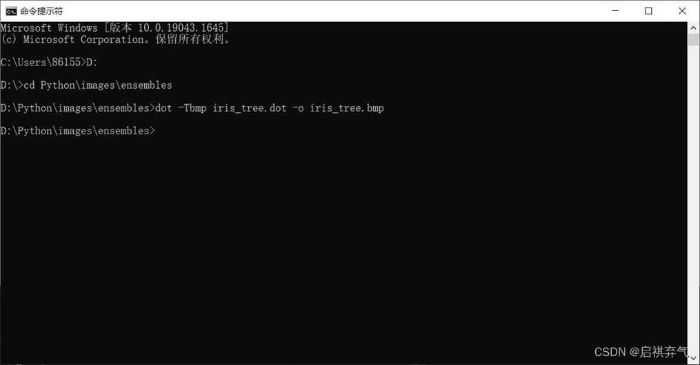
19. # 此处使用cmd将dot转换成pdf
20.
21. from matplotlib.colors import ListedColormap
22.
23.
24. def plot_decision_boundary(clf, X, y, axes=[0, 8, 0, 3], alpha=0.8, contour=True):
25. x1s = np.linspace(axes[0], axes[1], 100)
26. x2s = np.linspace(axes[2], axes[3], 100)
27. x1, x2 = np.meshgrid(x1s, x2s)
28. X_new = np.c_[x1.ravel(), x2.ravel(), x1.ravel(), x2.ravel()]
29. y_pred = clf.predict(X_new).reshape(x1.shape)
30. custom_cmap = ListedColormap(['#fafab0', '#9898ff', '#a0faa0'])
31. plt.contourf(x1, x2, y_pred, alpha=0.3, cmap=custom_cmap)
32. if contour:
33. custom_cmap2 = ListedColormap(['#7d7d58', '#4c4c7f', '#507d50'])
34. plt.contour(x1, x2, y_pred, cmap=custom_cmap2, alpha=0.8)
35. plt.plot(X[:, 2][y==0], X[:, 3][y==0], "yo", alpha=alpha, label="Iris setosa")
36. plt.plot(X[:, 2][y==1], X[:, 3][y==1], "bs", alpha=alpha, label="Iris versicolor")
37. plt.plot(X[:, 2][y==2], X[:, 3][y==2], "r^", alpha=alpha, label="Iris virginica")
38. plt.axis(axes)
39. plt.xlabel(r"$x_1$", fontsize=18)
40. plt.ylabel(r"$x_2$", fontsize=18, rotation=0)
41.
42.
43. plot_decision_boundary(tree_clf, X_train, y_train)
44. plt.xlabel("petal length/cm", fontsize=14)
45. plt.ylabel("petal width/cm", rotation='vertical', fontsize=14)
46. plt.title("decision tree decision boundaries plot", fontsize=16)
47. plt.text(1.40, 1.0, "Depth=0", fontsize=15)
48. plt.text(3.2, 1.80, "Depth=1", fontsize=13)
49. plt.text(4.05, 0.5, "Depth=2", fontsize=11)
50.
51. save_fig("decision_tree_decision_boundaries_plot")
52. plt.show()
4、在训练集上训练Boosting(基学习器:决策树)和随机森林模型,基学习器个数为100,输出决策边界图,并分析结果差异;
1.	from sklearn.ensemble import AdaBoostClassifier
2.	ada_clf = AdaBoostClassifier(
3.	    DecisionTreeClassifier(max_depth=4), n_estimators=100,
4.	    algorithm="SAMME.R", learning_rate=0.5, random_state=211)
5.	ada_clf.fit(X_train, y_train)
6.
7.
8.	def plot_decision_boundary(clf, X, y, axes=[0, 8, 0, 2.8], alpha=0.8, contour=True):
9.	    x1s = np.linspace(axes[0], axes[1], 100)
10.	    x2s = np.linspace(axes[2], axes[3], 100)
11.	    x1, x2 = np.meshgrid(x1s, x2s)
12.	    X_new = np.c_[x1.ravel(), x2.ravel(), x1.ravel(), x2.ravel()]
13.	    y_pred = clf.predict(X_new).reshape(x1.shape)
14.	    custom_cmap = ListedColormap(['#fafab0', '#9898ff', '#a0faa0'])
15.	    plt.contourf(x1, x2, y_pred, alpha=0.3, cmap=custom_cmap)
16.	    if contour:
17.	        custom_cmap2 = ListedColormap(['#7d7d58', '#4c4c7f', '#507d50'])
18.	        plt.contour(x1, x2, y_pred, cmap=custom_cmap2, alpha=0.8)
19.	    plt.plot(X[:, 2][y==0], X[:, 3][y==0], "yo", alpha=alpha, label="Iris setosa")
20.	    plt.plot(X[:, 2][y==1], X[:, 3][y==1], "bs", alpha=alpha, label="Iris versicolor")
21.	    plt.plot(X[:, 2][y==2], X[:, 3][y==2], "r^", alpha=alpha, label="Iris virginica")
22.	    plt.axis(axes)
23.	    plt.xlabel(r"$x_1$", fontsize=18)
24.	    plt.ylabel(r"$x_2$", fontsize=18, rotation=0)
25.
26.
27.	# 随机森林
28.	from sklearn.ensemble import RandomForestClassifier
29.	rnd_clf = RandomForestClassifier(n_estimators=100, random_state=211)
30.	rnd_clf.fit(X_train, y_train)
31.
32.	# 决策边界图绘制
33.	fig, axes = plt.subplots(ncols=2, figsize=(10, 2.7), sharey=True)
34.	plt.sca(axes[0])
35.	plot_decision_boundary(ada_clf, X, y)
36.	plt.xlabel("petal length/cm", fontsize=14)
37.	plt.ylabel("petal width/cm", rotation='vertical', fontsize=14)
38.	plt.title("boost决策边界 learning_rate=0.5 n_estimators=100",
39.	          fontsize=14)
40.
41.	plt.sca(axes[1])
42.	plot_decision_boundary(rnd_clf, X, y)
43.	plt.xlabel("petal length/cm", fontsize=14)
44.	plt.ylabel("petal width/cm", rotation='vertical', fontsize=14)
45.	plt.title("随机森林决策边界 n_estimators=100", fontsize=14)
46.	plt.suptitle("我是five", fontsize=16)
47.
48.	save_fig("Random_forest_decision_boundary_plot")
49.	plt.show()
5、分别计算决策树、Boosting(基学习器:决策树)和随机森林模型在Iris数据集上三分类的混淆矩阵,并对三种算法的输出结果进行比较。
1.	# 混淆矩阵
2.	from sklearn.metrics import confusion_matrix
3.	y_pre1 = tree_clf.predict(X_test)
4.	y_pre2 = ada_clf.predict(X_test)
5.	y_pre3 = rnd_clf.predict(X_test)
6.	confusion1 = confusion_matrix(y_test, y_pre1)
7.	confusion2 = confusion_matrix(y_test, y_pre2)
8.	confusion3 = confusion_matrix(y_test, y_pre3)
9.	print("决策树混淆矩阵 :\n",confusion1)
10.	print("Boosting混淆矩阵 :\n", confusion2)
11.	print("随机森林混淆矩阵 :\n", confusion3)
后记
随着学习的不断深入,我逐渐感觉我是five!而且我也辜负了我的会长小小鑫121,不好意思对面道歉,只好在这里道个歉,对不起!
附:源代码
4_ensemble_learning_and_random_forests.py
1.	# -*- coding: utf-8 -*-
2.	# Python ≥3.5 is required
3.	import sys
4.	assert sys.version_info >= (3, 5)
5.
6.	# Scikit-Learn ≥0.20 is required
7.	import sklearn
8.	assert sklearn.__version__ >= "0.20"
9.
10.	# Common imports
11.	import numpy as np
12.	import os
13.
14.	# to make this notebook's output stable across runs
15.	np.random.seed(211)
16.
17.	# To plot pretty figures
18.	import matplotlib as mpl
19.	import matplotlib.pyplot as plt
20.	plt.rcParams['font.sans-serif'] = ['Microsoft YaHei']
21.
22.	# Where to save the figures
23.	PROJECT_ROOT_DIR = "."
24.	CHAPTER_ID = "ensembles"
25.	IMAGES_PATH = os.path.join(PROJECT_ROOT_DIR, "images", CHAPTER_ID)
26.	os.makedirs(IMAGES_PATH, exist_ok=True)
27.
28.
29.	def save_fig(fig_id, tight_layout=True, fig_extension="png", resolution=300):
30.	    path = os.path.join(IMAGES_PATH, fig_id + "." + fig_extension)
31.	    print("Saving figure", fig_id)
32.	    if tight_layout:
33.	        plt.tight_layout()
34.	    plt.savefig(path, format=fig_extension, dpi=resolution)
35.
36.
37.	from sklearn.datasets import load_iris
38.	from sklearn.model_selection import train_test_split
39.
40.	iris = load_iris()
41.	X = iris.data
42.	y = iris.target
43.	X_train, X_test, y_train, y_test = train_test_split(X, y, test_size=0.3,
44.	                                                    random_state=211)
45.	print("训练集前十个数据:\n",np.c_[X_train[:10],y_train[:10]])
46.	print("测试集前十个数据:\n",np.c_[X_test[:10],y_test[:10]])
47.
48.	from sklearn.tree import DecisionTreeClassifier #决策树的分类器
49.	from graphviz import Source
50.	from sklearn.tree import export_graphviz
51.
52.	tree_clf = DecisionTreeClassifier(max_depth=4, random_state=211)  #决策树初始化
53.	tree_clf.fit(X_train, y_train)
54.	score = tree_clf.score(X_test, y_test)  # 训练集计算得分
55.
56.	export_graphviz(
57.	        tree_clf,
58.	        out_file=os.path.join(IMAGES_PATH, "iris_tree.dot"),
59.	        feature_names=iris.feature_names,
60.	        class_names=iris.target_names,
61.	        rounded=True,
62.	        filled=True
63.	    )
64.
65.	Source.from_file(os.path.join(IMAGES_PATH, "iris_tree.dot"))
66.	# 此处使用cmd将dot转换成pdf
67.
68.	from matplotlib.colors import ListedColormap
69.
70.
71.	def plot_decision_boundary(clf, X, y, axes=[0, 8, 0, 3], alpha=0.8, contour=True):
72.	    x1s = np.linspace(axes[0], axes[1], 100)
73.	    x2s = np.linspace(axes[2], axes[3], 100)
74.	    x1, x2 = np.meshgrid(x1s, x2s)
75.	    X_new = np.c_[x1.ravel(), x2.ravel(), x1.ravel(), x2.ravel()]
76.	    y_pred = clf.predict(X_new).reshape(x1.shape)
77.	    custom_cmap = ListedColormap(['#fafab0', '#9898ff', '#a0faa0'])
78.	    plt.contourf(x1, x2, y_pred, alpha=0.3, cmap=custom_cmap)
79.	    if contour:
80.	        custom_cmap2 = ListedColormap(['#7d7d58', '#4c4c7f', '#507d50'])
81.	        plt.contour(x1, x2, y_pred, cmap=custom_cmap2, alpha=0.8)
82.	    plt.plot(X[:, 2][y==0], X[:, 3][y==0], "yo", alpha=alpha, label="Iris setosa")
83.	    plt.plot(X[:, 2][y==1], X[:, 3][y==1], "bs", alpha=alpha, label="Iris versicolor")
84.	    plt.plot(X[:, 2][y==2], X[:, 3][y==2], "r^", alpha=alpha, label="Iris virginica")
85.	    plt.axis(axes)
86.	    plt.xlabel(r"$x_1$", fontsize=18)
87.	    plt.ylabel(r"$x_2$", fontsize=18, rotation=0)
88.
89.
90.	plot_decision_boundary(tree_clf, X_train, y_train)
91.	plt.xlabel("petal length/cm", fontsize=14)
92.	plt.ylabel("petal width/cm", rotation='vertical', fontsize=14)
93.	plt.title("decision tree decision boundaries plot\n高啟祺 电信1904 0121909361211", fontsize=16)
94.	plt.text(1.40, 1.0, "Depth=0", fontsize=15)
95.	plt.text(3.2, 1.80, "Depth=1", fontsize=13)
96.	plt.text(4.05, 0.5, "Depth=2", fontsize=11)
97.
98.	save_fig("decision_tree_decision_boundaries_plot")
99.	plt.show()
100.
101.	from sklearn.ensemble import AdaBoostClassifier
102.	ada_clf = AdaBoostClassifier(
103.	    DecisionTreeClassifier(max_depth=4), n_estimators=100,
104.	    algorithm="SAMME.R", learning_rate=0.5, random_state=211)
105.	ada_clf.fit(X_train, y_train)
106.
107.
108.	def plot_decision_boundary(clf, X, y, axes=[0, 8, 0, 2.8], alpha=0.8, contour=True):
109.	    x1s = np.linspace(axes[0], axes[1], 100)
110.	    x2s = np.linspace(axes[2], axes[3], 100)
111.	    x1, x2 = np.meshgrid(x1s, x2s)
112.	    X_new = np.c_[x1.ravel(), x2.ravel(), x1.ravel(), x2.ravel()]
113.	    y_pred = clf.predict(X_new).reshape(x1.shape)
114.	    custom_cmap = ListedColormap(['#fafab0', '#9898ff', '#a0faa0'])
115.	    plt.contourf(x1, x2, y_pred, alpha=0.3, cmap=custom_cmap)
116.	    if contour:
117.	        custom_cmap2 = ListedColormap(['#7d7d58', '#4c4c7f', '#507d50'])
118.	        plt.contour(x1, x2, y_pred, cmap=custom_cmap2, alpha=0.8)
119.	    plt.plot(X[:, 2][y==0], X[:, 3][y==0], "yo", alpha=alpha, label="Iris setosa")
120.	    plt.plot(X[:, 2][y==1], X[:, 3][y==1], "bs", alpha=alpha, label="Iris versicolor")
121.	    plt.plot(X[:, 2][y==2], X[:, 3][y==2], "r^", alpha=alpha, label="Iris virginica")
122.	    plt.axis(axes)
123.	    plt.xlabel(r"$x_1$", fontsize=18)
124.	    plt.ylabel(r"$x_2$", fontsize=18, rotation=0)
125.
126.
127.	# 随机森林
128.	from sklearn.ensemble import RandomForestClassifier
129.	rnd_clf = RandomForestClassifier(n_estimators=100, random_state=211)
130.	rnd_clf.fit(X_train, y_train)
131.
132.	# 决策边界图绘制
133.	fig, axes = plt.subplots(ncols=2, figsize=(10, 2.7), sharey=True)
134.	plt.sca(axes[0])
135.	plot_decision_boundary(ada_clf, X, y)
136.	plt.xlabel("petal length/cm", fontsize=14)
137.	plt.ylabel("petal width/cm", rotation='vertical', fontsize=14)
138.	plt.title("boost决策边界 learning_rate=0.5 n_estimators=100",
139.	          fontsize=14)
140.
141.	plt.sca(axes[1])
142.	plot_decision_boundary(rnd_clf, X, y)
143.	plt.xlabel("petal length/cm", fontsize=14)
144.	plt.ylabel("petal width/cm", rotation='vertical', fontsize=14)
145.	plt.title("随机森林决策边界 n_estimators=100", fontsize=14)
146.	plt.suptitle("高啟祺 电信1904 0121909361211", fontsize=16)
147.
148.	save_fig("Random_forest_decision_boundary_plot")
149.	plt.show()
150.
151.	# 混淆矩阵
152.	from sklearn.metrics import confusion_matrix
153.	y_pre1 = tree_clf.predict(X_test)
154.	y_pre2 = ada_clf.predict(X_test)
155.	y_pre3 = rnd_clf.predict(X_test)
156.	confusion1 = confusion_matrix(y_test, y_pre1)
157.	confusion2 = confusion_matrix(y_test, y_pre2)
158.	confusion3 = confusion_matrix(y_test, y_pre3)
159.	print("决策树混淆矩阵 :\n",confusion1)
160.	print("Boosting混淆矩阵 :\n", confusion2)
161.	print("随机森林混淆矩阵 :\n", confusion3)

CSDN联合极客时间,共同打造面向开发者的精品内容学习社区,助力成长!
更多推荐


 0
0 0
0- 0


 已为社区贡献2条内容

所有评论(0)